How to compute Z-score
Introduction
A Z-score measures how many standard deviations a data point is from the mean, allowing you to standardize values across different scales. This is essential for comparing data points from different distributions, identifying outliers, and preparing data for statistical analyses that assume standardized inputs.
Getting Started
library(tidyverse)
library(palmerpenguins)
Example 1: Basic Usage
The Problem
We need to calculate Z-scores for penguin body mass to understand which penguins are unusually heavy or light. This will help us identify outliers and standardize the measurements.
Step 1: Prepare the data
First, let’s examine our dataset and remove any missing values.
# Load and inspect penguin data
data("penguins")
clean_penguins <- penguins |>
  filter(!is.na(body_mass_g)) |>
  select(species, body_mass_g)

head(clean_penguins)
We now have clean data with 342 penguins and their body masses ready for Z-score calculation.
Step 2: Calculate Z-scores manually
We’ll compute Z-scores using the formula: (value - mean) / standard deviation.
# Calculate mean and standard deviation
mass_mean <- mean(clean_penguins$body_mass_g)
mass_sd <- sd(clean_penguins$body_mass_g)

# Compute Z-scores
clean_penguins$z_score <- (clean_penguins$body_mass_g - mass_mean) / mass_sd
Each penguin now has a Z-score showing how many standard deviations their mass is from the average.
Step 3: Interpret the results
Let’s examine the Z-scores to understand what they tell us.
# View penguins with extreme Z-scores
extreme_penguins <- clean_penguins |>
  filter(abs(z_score) > 2) |>
  arrange(desc(z_score))

print(extreme_penguins)
Penguins with Z-scores above 2 or below -2 are unusually heavy or light, representing less than 5% of the population.
Example 2: Practical Application
The Problem
We want to compare body mass across different penguin species by standardizing within each group. This allows us to identify which individual penguins are outliers within their own species, rather than compared to all penguins combined.
Step 1: Group-wise Z-score calculation
We’ll calculate Z-scores separately for each species using group operations.
# Calculate Z-scores within each species
penguins_grouped <- clean_penguins |>
  group_by(species) |>
  mutate(
    species_mean = mean(body_mass_g),
    species_sd = sd(body_mass_g)
  )
Now each penguin has their species-specific mean and standard deviation for comparison.
Step 2: Compute species-standardized Z-scores
We’ll create Z-scores that show how unusual each penguin is within its own species.
# Calculate within-species Z-scores
penguins_grouped <- penguins_grouped |>
  mutate(
    species_z_score = (body_mass_g - species_mean) / species_sd
  ) |>
  ungroup()
These species-specific Z-scores reveal which penguins are outliers relative to their own kind.
Step 3: Compare overall vs species-specific outliers
Let’s identify penguins that are outliers in different contexts.
# Find different types of outliers
outlier_comparison <- penguins_grouped |>
  mutate(
    overall_outlier = abs(z_score) > 2,
    species_outlier = abs(species_z_score) > 2
  ) |>
  select(species, body_mass_g, z_score, species_z_score,
         overall_outlier, species_outlier)
This comparison reveals how standardization context affects outlier identification.
Step 4: Visualize the differences
Create a visualization to show both standardization approaches.
# Create comparison plot
ggplot(penguins_grouped, aes(x = species, y = species_z_score, fill = species)) +
  geom_boxplot(alpha = 0.7) +
  geom_hline(yintercept = c(-2, 2), linetype = "dashed", color = "red") +
  labs(title = "Species-Standardized Z-scores",
       x = "Species",
       y = "Z-score within species")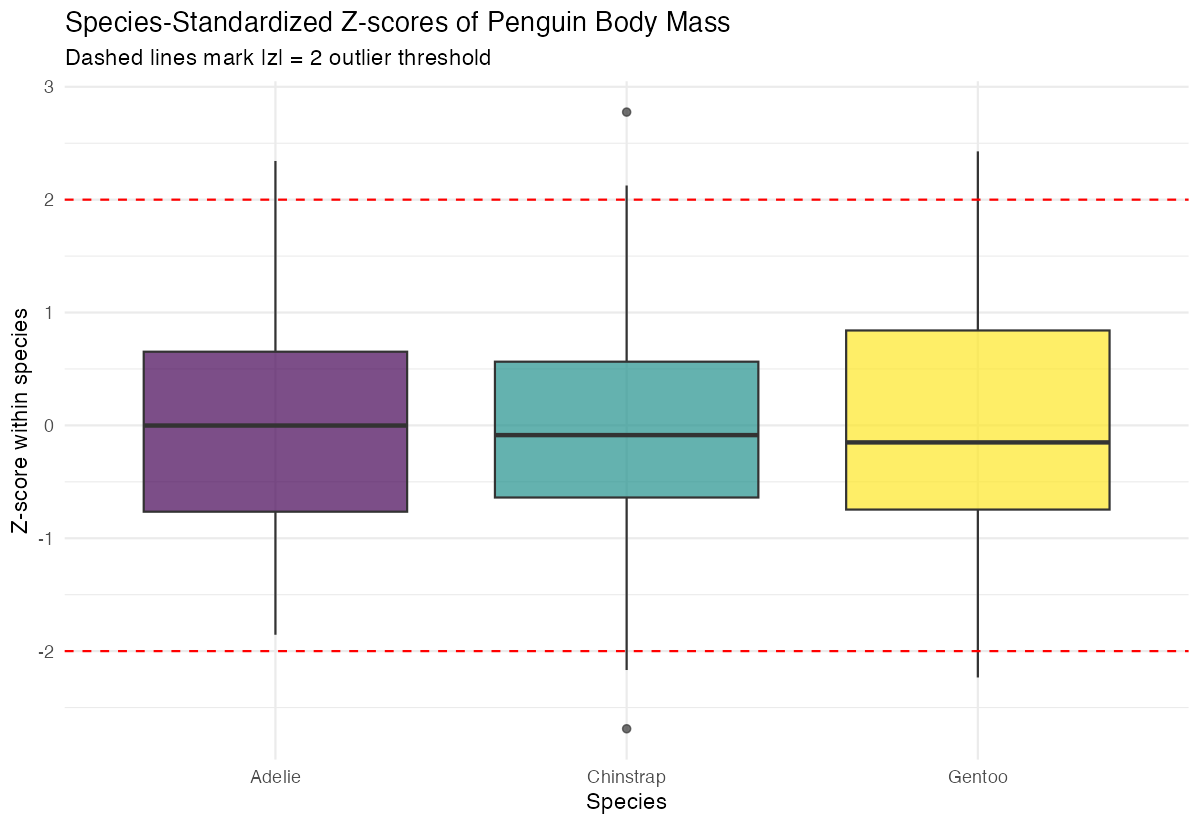
The plot shows that each species now has a similar distribution of Z-scores, making cross-species comparisons more meaningful.
Summary
- Z-scores standardize data by measuring distance from the mean in standard deviation units
- Calculate Z-scores using the formula: (value - mean) / standard deviation
- Values with absolute Z-scores greater than 2 are typically considered outliers
- Group-wise Z-scores allow meaningful comparisons within subgroups of your data
Choose between overall or group-specific standardization based on your analysis goals