How to paired t-test in R
Introduction
A paired t-test compares the means of two related groups to determine if there’s a statistically significant difference between them. This test is used when you have paired observations, such as before-and-after measurements on the same subjects or matched pairs in experimental design.
Getting Started
library(tidyverse)
library(palmerpenguins)
Example 1: Basic Usage
The Problem
We want to test if there’s a significant difference between flipper length measurements taken by two different researchers on the same penguins. This simulates a paired design where each penguin is measured twice.
Step 1: Prepare the Data
We’ll create paired measurements by adding measurement error to simulate two researchers.
set.seed(123)
penguins_clean <- penguins |>
  filter(!is.na(flipper_length_mm)) |>
  slice_head(n = 50)

paired_data <- penguins_clean |>
  mutate(researcher_1 = flipper_length_mm,
         researcher_2 = flipper_length_mm + rnorm(50, mean = 2, sd = 3))
This creates our paired dataset with measurements from two researchers on the same 50 penguins.
Step 2: Visualize the Paired Data
Let’s examine the relationship between the paired measurements.
paired_data |>
  ggplot(aes(x = researcher_1, y = researcher_2)) +
  geom_point(size = 2, alpha = 0.8, color = "steelblue") +
  geom_abline(intercept = 0, slope = 1, color = "red", linetype = "dashed",
              linewidth = 1) +
  labs(title = "Paired Flipper Length Measurements by Two Researchers",
       subtitle = "Red dashed line shows perfect agreement (y = x)",
       x = "Researcher 1 (mm)", y = "Researcher 2 (mm)")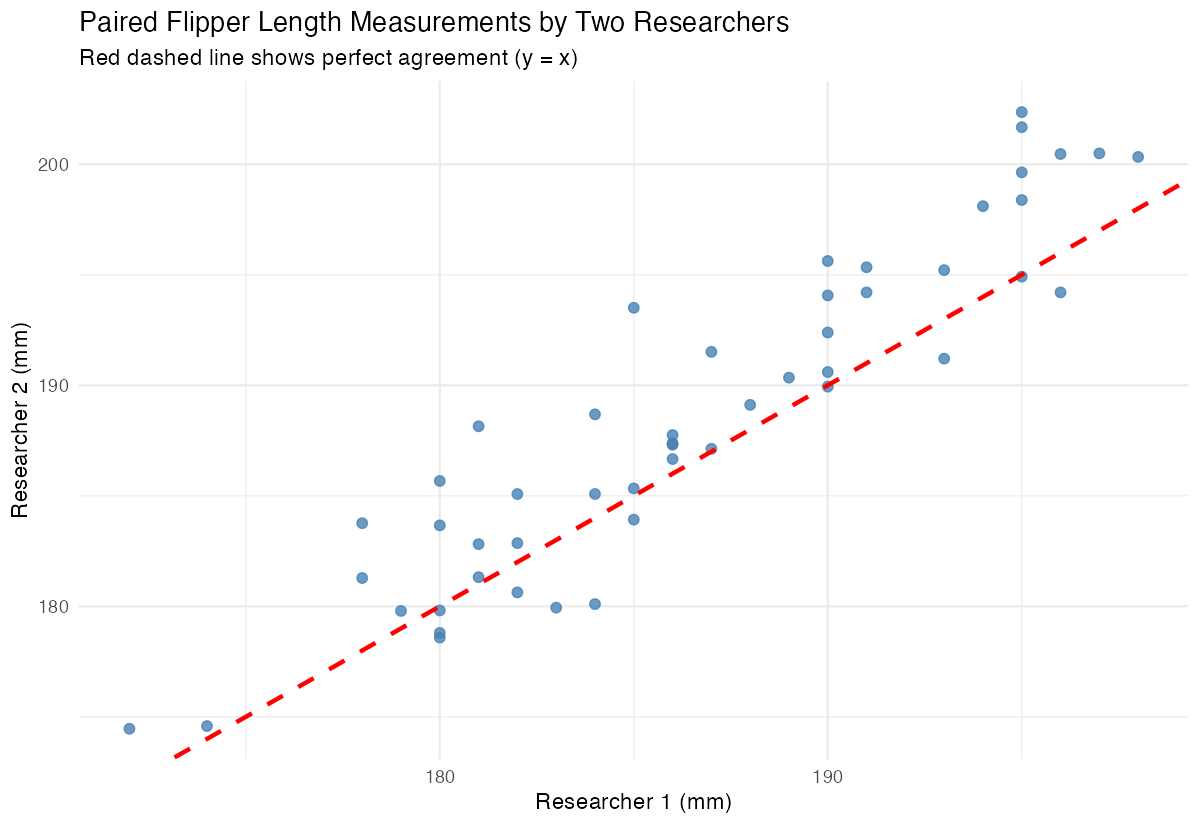
The scatter plot shows how the paired measurements relate to each other, with the red line indicating perfect agreement.
Step 3: Perform the Paired t-test
Now we’ll conduct the paired t-test using the built-in function.
t_test_result <- t.test(paired_data$researcher_1,
                       paired_data$researcher_2,
                       paired = TRUE)
print(t_test_result)
The paired t-test compares the mean difference between the two measurements and tests if it’s significantly different from zero.
Step 4: Calculate Differences Manually
Understanding what happens behind the scenes helps interpret results.
differences <- paired_data$researcher_1 - paired_data$researcher_2
mean_diff <- mean(differences)
se_diff <- sd(differences) / sqrt(length(differences))

cat("Mean difference:", round(mean_diff, 2), "\n")
cat("Standard error:", round(se_diff, 2))
This shows the mean difference and its standard error, which are the foundation of the t-test calculation.
Example 2: Practical Application
The Problem
A fitness trainer wants to test if a 6-week training program improves performance. We’ll simulate before-and-after body mass measurements to see if the program leads to significant weight loss in penguins during breeding season.
Step 1: Create Before-After Data
We’ll simulate a realistic scenario with weight measurements.
set.seed(456)
fitness_data <- penguins |>
  filter(!is.na(body_mass_g)) |>
  slice_head(n = 30) |>
  mutate(before = body_mass_g,
         after = body_mass_g - abs(rnorm(30, mean = 150, sd = 100)))
This creates before-and-after weight measurements for 30 penguins in our fitness study.
Step 2: Explore the Data Distribution
Let’s examine the distribution of differences before testing.
fitness_data <- fitness_data |>
  mutate(weight_loss = before - after)

fitness_data |>
  ggplot(aes(x = weight_loss)) +
  geom_histogram(bins = 10, fill = "lightblue", alpha = 0.8, color = "black") +
  labs(title = "Distribution of Weight Loss (Before - After)",
       subtitle = "Paired differences used in the t-test",
       x = "Weight Loss (g)", y = "Count")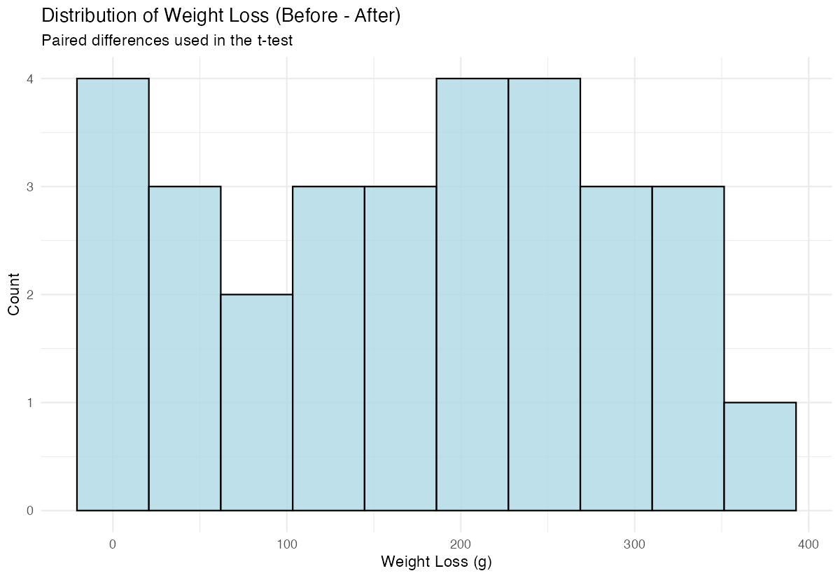
The histogram shows us the distribution of weight changes, helping us assess if the data looks reasonable for a t-test.
Step 3: Conduct the Paired t-test
Now we’ll test if the weight loss is statistically significant.
fitness_test <- t.test(fitness_data$before,
                      fitness_data$after,
                      paired = TRUE,
                      alternative = "greater")
print(fitness_test)
We use alternative = "greater" because we expect the before weights to be greater than after weights.
Step 4: Interpret and Visualize Results
Let’s create a visual summary of our findings.
fitness_data |>
  mutate(id = row_number()) |>
  select(id, before, after) |>
  pivot_longer(cols = c(before, after),
               names_to = "period", values_to = "weight") |>
  mutate(period = factor(period, levels = c("before", "after"))) |>
  ggplot(aes(x = period, y = weight, group = id)) +
  geom_line(alpha = 0.4, color = "steelblue", linewidth = 0.6) +
  geom_point(alpha = 0.8, color = "steelblue", size = 2) +
  labs(title = "Paired Before vs After Weight Measurements",
       subtitle = "Each line connects one penguin's paired observations",
       x = "Period", y = "Body Mass (g)")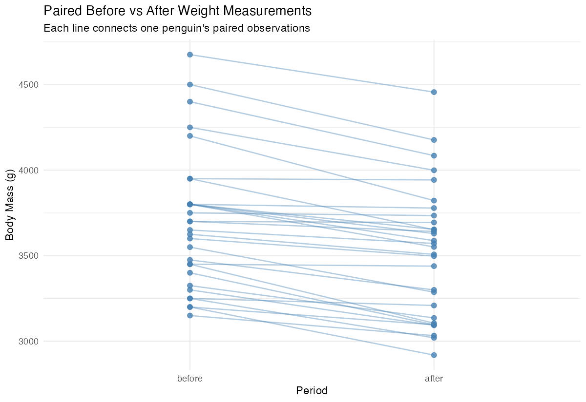
This visualization shows individual changes for each penguin, making the paired nature of our data clear.
Summary
- Paired t-tests compare means of two related groups using the same subjects or matched pairs
- Use
t.test(x, y, paired = TRUE)for the basic paired t-test in R - Always visualize your paired data to understand the relationship and check assumptions
- The test actually analyzes the differences between pairs, testing if the mean difference equals zero
Consider the direction of your hypothesis when setting the
alternativeparameter (“two.sided”, “greater”, or “less”)