How to t-test for two samples in R
Introduction
A two-sample t-test is a statistical method used to determine whether there is a significant difference between the means of two independent groups. This test is fundamental in comparing populations and is widely used across various fields including biology, psychology, business, and healthcare.
You would use a two-sample t-test when you have continuous data from two separate groups and want to test if their population means are significantly different. For example, comparing test scores between two teaching methods, analyzing weight differences between male and female animals, or evaluating performance metrics between two product versions. The test assumes that both groups follow approximately normal distributions and have similar variances.
Getting Started
First, let’s load the necessary packages for our analysis:
library(tidyverse)
library(palmerpenguins)
Example 1: Basic Usage
Let’s start with a simple example using the built-in mtcars dataset to compare fuel efficiency between automatic and manual transmission cars:
data(mtcars)

automatic <- mtcars$mpg[mtcars$am == 0]
manual <- mtcars$mpg[mtcars$am == 1]

t.test(automatic, manual)
We can also perform the same test using formula syntax, which is often more intuitive:
t.test(mpg ~ am, data = mtcars)To specify a one-tailed test (if we hypothesize that manual cars have better fuel efficiency):
t.test(mpg ~ am, data = mtcars, alternative = "less")Example 2: Practical Application
Now let’s explore a more comprehensive example using the Palmer Penguins dataset. We’ll compare flipper lengths between Adelie and Chinstrap penguins:
data(penguins)

penguin_comparison <- penguins |>
  filter(species %in% c("Adelie", "Chinstrap")) |>
  drop_na(flipper_length_mm)

penguin_comparison |>
  group_by(species) |>
  summarise(
    count = n(),
    mean_flipper = mean(flipper_length_mm),
    sd_flipper = sd(flipper_length_mm)
  )

t_test_result <- t.test(flipper_length_mm ~ species, data = penguin_comparison)
print(t_test_result)
Let’s also check our assumptions before interpreting the results:
adelie_flippers <- penguin_comparison |>
  filter(species == "Adelie") |>
  pull(flipper_length_mm)

chinstrap_flippers <- penguin_comparison |>
  filter(species == "Chinstrap") |>
  pull(flipper_length_mm)

var.test(adelie_flippers, chinstrap_flippers)
If variances are significantly different, we can use Welch’s t-test (which is actually the default in R):
t.test(flipper_length_mm ~ species,
       data = penguin_comparison,
       var.equal = FALSE)
For a more complete analysis, let’s create a visualization to accompany our statistical test:
penguin_comparison |>
  ggplot(aes(x = species, y = flipper_length_mm, fill = species)) +
  geom_boxplot(alpha = 0.7, outlier.shape = NA) +
  geom_jitter(width = 0.2, alpha = 0.6) +
  labs(
    title = "Flipper Length Comparison: Adelie vs Chinstrap Penguins",
    subtitle = "Two-sample t-test of flipper length by species",
    x = "Species",
    y = "Flipper Length (mm)",
    caption = paste("t-test p-value:", round(t_test_result$p.value, 4))
  ) +
  theme_minimal() +
  theme(legend.position = "none")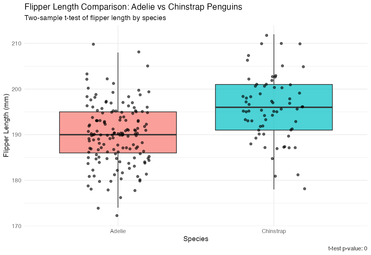
We can also perform a one-sample t-test to compare against a hypothetical population mean:
adelie_flippers <- penguins |>
  filter(species == "Adelie") |>
  pull(flipper_length_mm) |>
  na.omit()

t.test(adelie_flippers, mu = 190)
Summary
Two-sample t-tests are powerful tools for comparing means between groups. Key takeaways include:
- Use
t.test(x, y)for vectors ort.test(y ~ x, data)for formula syntax - The default Welch’s t-test doesn’t assume equal variances, making it more robust
- Always check assumptions: normality and independence of observations
- Combine statistical tests with visualizations for better interpretation
- Consider the practical significance of differences, not just statistical significance