How to z-score normalization in R
Introduction
Z-score normalization (also called standardization) transforms data to have a mean of 0 and standard deviation of 1. This technique converts raw values into standardized scores that represent how many standard deviations a value is from the mean.
Z-score normalization is essential when working with variables measured on different scales, preparing data for machine learning algorithms, identifying outliers, or comparing values across different distributions. For example, if you’re analyzing penguin body measurements, z-scores help compare flipper length (measured in millimeters) with body mass (measured in grams) on the same standardized scale.
The formula is: z = (x - μ) / σ, where x is the original value, μ is the mean, and σ is the standard deviation.
Getting Started
library(tidyverse)
library(palmerpenguins)
Example 1: Basic Z-Score Normalization
Let’s start with a simple example using the scale() function, which is the most straightforward way to z-score normalize data in R:
# Create sample data
sample_data <- c(10, 15, 20, 25, 30, 35, 40)

# Z-score normalization using scale()
z_scores <- scale(sample_data)
print(z_scores)

# Verify the results
mean(z_scores)
sd(z_scores)

# Manual calculation for comparison
manual_z <- (sample_data - mean(sample_data)) / sd(sample_data)
print(manual_z)
You can also create your own z-score function:
z_normalize <- function(x) {
  (x - mean(x, na.rm = TRUE)) / sd(x, na.rm = TRUE)
}

# Apply custom function
custom_z_scores <- z_normalize(sample_data)
print(custom_z_scores)
Example 2: Practical Application with Palmer Penguins
Let’s apply z-score normalization to real data using the Palmer penguins dataset. This example shows how to normalize multiple variables and compare penguins across different measurement scales:
# Load and explore the data
data(penguins)
head(penguins)

# Z-score normalize numeric variables
penguins_normalized <- penguins |>
  filter(!is.na(bill_length_mm)) |>
  mutate(
    bill_length_z = scale(bill_length_mm)[,1],
    bill_depth_z = scale(bill_depth_mm)[,1],
    flipper_length_z = scale(flipper_length_mm)[,1],
    body_mass_z = scale(body_mass_g)[,1]
  )

# View the normalized data
penguins_normalized |>
  select(species, bill_length_mm, bill_length_z, body_mass_g, body_mass_z) |>
  head(10)
Now let’s normalize variables by species groups, which is often more meaningful for comparative analysis:
# Z-score normalize within each species
penguins_by_species <- penguins |>
  filter(!is.na(bill_length_mm)) |>
  group_by(species) |>
  mutate(
    bill_length_z = scale(bill_length_mm)[,1],
    bill_depth_z = scale(bill_depth_mm)[,1],
    flipper_length_z = scale(flipper_length_mm)[,1],
    body_mass_z = scale(body_mass_g)[,1]
  ) |>
  ungroup()

# Compare original vs normalized values
comparison <- penguins_by_species |>
  select(species, bill_length_mm, bill_length_z, body_mass_g, body_mass_z) |>
  arrange(species)

print(comparison)
Let’s visualize the effect of normalization:
# Create comparison plots
library(patchwork)

# Original data
p1 <- penguins |>
  filter(!is.na(bill_length_mm)) |>
  ggplot(aes(x = bill_length_mm, y = body_mass_g, color = species)) +
  geom_point() +
  labs(title = "Original Data", x = "Bill Length (mm)", y = "Body Mass (g)")

# Normalized data
p2 <- penguins_normalized |>
  ggplot(aes(x = bill_length_z, y = body_mass_z, color = species)) +
  geom_point() +
  labs(title = "Z-Score Normalized", x = "Bill Length (z-score)", y = "Body Mass (z-score)")

# Display plots side by side
p1 / p2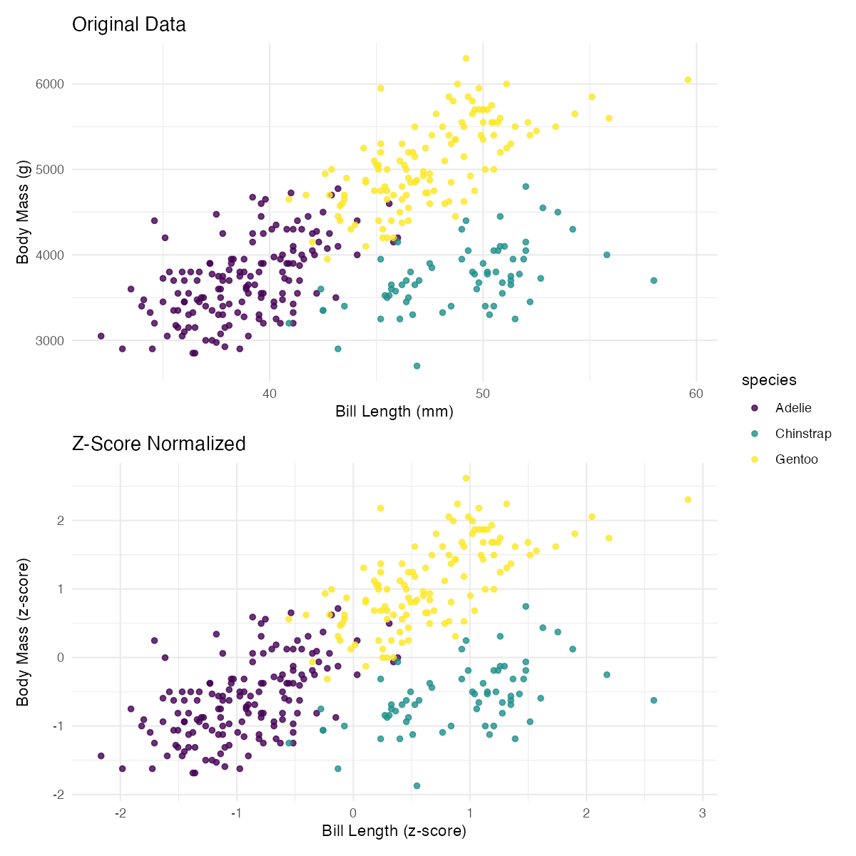
For multiple variables at once, use across():
# Normalize all numeric columns at once
penguins_all_normalized <- penguins |>
  mutate(across(where(is.numeric), ~ scale(.x)[,1], .names = "{.col}_z"))

# View the results
penguins_all_normalized |>
  select(species, ends_with("_z")) |>
  head()
Summary
Z-score normalization is a fundamental data preprocessing technique that standardizes variables to have mean = 0 and standard deviation = 1. Key takeaways include:
- Use
scale()for quick z-score normalization of single variables - The
[,1]notation converts the matrix output ofscale()to a vector - Apply normalization within groups using
group_by()when comparing across categories - Use
across()withwhere(is.numeric)to normalize multiple columns efficiently - Always handle missing values appropriately with
na.rm = TRUEin custom functions