Logistic Regression with Single Predictor in R
Introduction
Logistic regression is used when you want to predict a binary outcome (yes/no, success/failure) based on one predictor variable. Unlike linear regression, it models the probability of an event occurring using the logistic function, which ensures predictions stay between 0 and 1.
Getting Started
library(tidyverse)
library(palmerpenguins)
Example 1: Basic Usage
The Problem
We want to predict whether a penguin is from the Adelie species based on its bill length. This is a binary classification problem where we’re modeling the probability of being Adelie versus not Adelie.
Step 1: Prepare the Data
We’ll create a binary outcome variable and examine our data structure.
penguins_clean <- penguins |>
  filter(!is.na(bill_length_mm), !is.na(species)) |>
  mutate(is_adelie = ifelse(species == "Adelie", 1, 0))

head(penguins_clean)
We now have a dataset with a binary variable is_adelie where 1 means Adelie and 0 means other species.
Step 2: Visualize the Relationship
Before modeling, let’s see how bill length relates to species.
ggplot(penguins_clean, aes(x = bill_length_mm, y = is_adelie)) +
  geom_point(alpha = 0.6) +
  geom_smooth(method = "glm", method.args = list(family = "binomial")) +
  labs(x = "Bill Length (mm)", y = "Probability of being Adelie")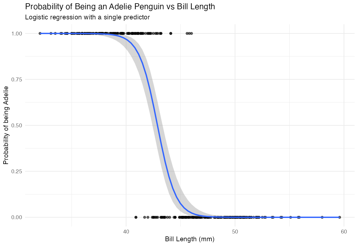
The smooth curve shows the logistic relationship - shorter bills are associated with higher probability of being Adelie.
Step 3: Fit the Logistic Model
We use glm() with family = “binomial” to fit our logistic regression.
model <- glm(is_adelie ~ bill_length_mm,
            data = penguins_clean,
            family = binomial)

summary(model)
The negative coefficient indicates that as bill length increases, the probability of being Adelie decreases.
Step 4: Make Predictions
Let’s predict probabilities for specific bill lengths.
new_data <- data.frame(bill_length_mm = c(35, 40, 45, 50))
predictions <- predict(model, new_data, type = "response")
data.frame(bill_length = new_data$bill_length_mm,
          probability_adelie = round(predictions, 3))
These probabilities show how bill length affects the likelihood of a penguin being Adelie.
Example 2: Practical Application
The Problem
A researcher wants to determine if a car’s weight can predict whether it has high fuel efficiency (mpg > 20). This helps understand the relationship between vehicle weight and fuel economy for purchasing decisions.
Step 1: Create Binary Outcome
We’ll transform the continuous mpg variable into a binary high/low efficiency indicator.
mtcars_binary <- mtcars |>
  mutate(high_mpg = ifelse(mpg > 20, 1, 0))

table(mtcars_binary$high_mpg)
We have 14 cars with high efficiency (>20 mpg) and 18 with lower efficiency.
Step 2: Explore the Data
Let’s visualize how weight relates to fuel efficiency.
ggplot(mtcars_binary, aes(x = wt, y = high_mpg)) +
  geom_point() +
  geom_smooth(method = "glm", method.args = list(family = "binomial")) +
  labs(x = "Weight (1000 lbs)", y = "Probability of High MPG")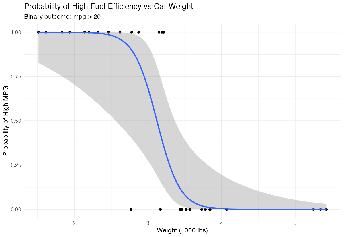
Heavier cars clearly have lower probability of achieving high fuel efficiency.
Step 3: Build the Model
We fit a logistic regression to quantify this relationship.
weight_model <- glm(high_mpg ~ wt,
                   data = mtcars_binary,
                   family = binomial)

summary(weight_model)
The significant negative coefficient confirms that weight strongly predicts lower fuel efficiency.
Step 4: Calculate Odds Ratios
Odds ratios help interpret the practical impact of weight changes.
exp(coef(weight_model))
exp(confint(weight_model))
For each additional 1000 lbs, the odds of high fuel efficiency multiply by this factor (less than 1 means decreased odds).
Step 5: Evaluate Model Performance
We’ll check how well our model classifies cars.
predicted_probs <- predict(weight_model, type = "response")
predicted_class <- ifelse(predicted_probs > 0.5, 1, 0)
confusion_matrix <- table(Actual = mtcars_binary$high_mpg,
                         Predicted = predicted_class)
print(confusion_matrix)
This confusion matrix shows our model’s accuracy in predicting high versus low fuel efficiency.
Summary
- Logistic regression models binary outcomes using predictor variables and the logistic function
- Use
glm()withfamily = binomialto fit logistic regression models in R - Coefficients represent changes in log-odds; negative coefficients decrease probability of success
- Convert coefficients using
exp()to get odds ratios for easier interpretation Always visualize your data first and evaluate model performance with predicted probabilities