List of Built in Datasets in R
Introduction
R comes with numerous built-in datasets that are perfect for learning, testing code, and exploring statistical methods without needing to import external data. These datasets are immediately available in your R session and cover various domains from economics to biology, making them invaluable for data science practice and education.
Getting Started
library(tidyverse)
library(palmerpenguins)
Example 1: Basic Usage
The Problem
You need to quickly access sample data for testing your analysis code or learning new functions. Finding and loading external datasets can be time-consuming when you just want to practice data manipulation techniques.
Step 1: View Available Datasets
Start by exploring what datasets are available in your R installation.
# See all built-in datasets
data()

# View datasets from specific package
data(package = "datasets")
This opens a window showing all available datasets with brief descriptions of each one.
Step 2: Load a Dataset
Load the famous mtcars dataset to begin exploration.
# Load mtcars dataset
data(mtcars)

# Quick overview
head(mtcars)
glimpse(mtcars)
The dataset is now loaded in your environment with 32 car models and 11 variables including mpg, horsepower, and weight.
Step 3: Basic Dataset Information
Get essential information about the dataset structure and contents.
# Dataset dimensions and structure
dim(mtcars)
names(mtcars)
summary(mtcars)
This reveals mtcars has 32 rows and 11 columns, showing summary statistics for each numeric variable.
Example 2: Practical Application
The Problem
You’re teaching a data visualization workshop and need engaging, real-world datasets that participants can immediately start analyzing. The penguins dataset provides rich biological data perfect for demonstrating various plot types and statistical concepts.
Step 1: Load and Explore Penguins Data
Access the palmerpenguins dataset for biological analysis.
# Load penguins data
data(penguins)

# Examine structure
str(penguins)
head(penguins, 3)
The penguins dataset contains 344 observations of Antarctic penguins with species, island, and physical measurements.
Step 2: Quick Data Analysis
Perform basic exploratory analysis using the loaded dataset.
# Summary by species
penguins |>
  group_by(species) |>
  summarise(
    count = n(),
    avg_mass = mean(body_mass_g, na.rm = TRUE)
  )
This shows three penguin species with Gentoo penguins being the heaviest on average at about 5,076 grams.
Step 3: Create Visualizations
Generate plots immediately without data import hassles.
# Scatter plot of bill dimensions
penguins |>
  ggplot(aes(bill_length_mm, bill_depth_mm, color = species)) +
  geom_point() +
  labs(title = "Penguin Bill Dimensions by Species")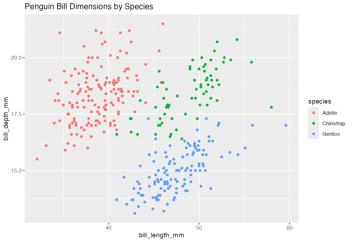
The visualization clearly shows distinct clustering by species, with each having different bill characteristics.
Step 4: Advanced Analysis
Combine multiple built-in datasets for comparative analysis.
# Quick correlation analysis
mtcars |>
  select(mpg, hp, wt, qsec) |>
  cor() |>
  round(2)
This correlation matrix reveals strong negative relationships between fuel efficiency (mpg) and both horsepower and weight.
Summary
- Built-in datasets like mtcars, iris, and penguins provide immediate access to quality data for analysis and learning
- Use
data()to view all available datasets anddata(dataset_name)to load specific ones into your environment
- These datasets are perfect for testing code, creating tutorials, and practicing new statistical techniques without setup time
- Popular datasets include mtcars (automotive), penguins (biology), economics (time series), and diamonds (gemology)
Built-in datasets save time in educational settings and allow focus on analysis techniques rather than data preparation