How to Compute Compound Interest with Tidyverse
Compound interest calculations are essential for financial planning and investment analysis. The tidyverse provides powerful tools for computing compound interest across different time periods and scenarios, making it easy to visualize and compare investment growth.
Getting Started
library(tidyverse)
library(palmerpenguins)
Example 1: Basic Compound Interest Calculation
The Problem
You want to calculate how a $1000 investment grows over 10 years with 7% annual interest. We need to compute the compound interest formula: A = P(1 + r)^t.
Step 1: Create the Investment Data
We’ll start by setting up our basic investment parameters.
investment <- tibble(
  principal = 1000,
  rate = 0.07,
  years = 10
)
This creates a data frame with our initial investment amount, interest rate, and time period.
Step 2: Calculate Final Amount
Now we’ll apply the compound interest formula using mutate().
investment <- investment |>
  mutate(
    final_amount = principal * (1 + rate)^years,
    total_interest = final_amount - principal
  )
The investment grows to $1967.15 with $967.15 in compound interest earned.
Step 3: View the Results
Let’s examine our calculation results.
investment |>
  select(principal, final_amount, total_interest) |>
  mutate(across(where(is.numeric), ~ round(.x, 2)))
This shows the principal, final amount, and total interest earned in a clean format.
Example 2: Comparing Multiple Investment Scenarios
The Problem
You want to compare different investment strategies with varying principals, interest rates, and time periods. This helps you understand how different factors affect compound growth and make informed investment decisions.
Step 1: Create Multiple Scenarios
We’ll set up different investment scenarios to compare.
scenarios <- tibble(
  scenario = c("Conservative", "Moderate", "Aggressive"),
  principal = c(5000, 10000, 15000),
  annual_rate = c(0.04, 0.07, 0.10),
  years = c(20, 15, 10)
)
Each scenario represents a different risk-return profile with varying investment amounts and rates.
Step 2: Calculate Growth Over Time
Now we’ll expand each scenario to show year-by-year growth.
yearly_growth <- scenarios |>
  rowwise() |>
  mutate(
    year_data = list(1:years),
    .keep = "all"
  ) |>
  unnest(year_data)
This creates a row for each year in each investment scenario for detailed tracking.
Step 3: Compute Annual Values
We’ll calculate the investment value for each year.
yearly_growth <- yearly_growth |>
  mutate(
    amount = principal * (1 + annual_rate)^year_data,
    interest_earned = amount - principal
  )
Now we have the compound growth calculated for each year across all scenarios.
Step 4: Visualize the Growth
Let’s create a visualization to compare the scenarios.
yearly_growth |>
  ggplot(aes(x = year_data, y = amount, color = scenario)) +
  geom_line(size = 1.2) +
  labs(title = "Compound Interest Growth Comparison",
       x = "Years", y = "Investment Value ($)")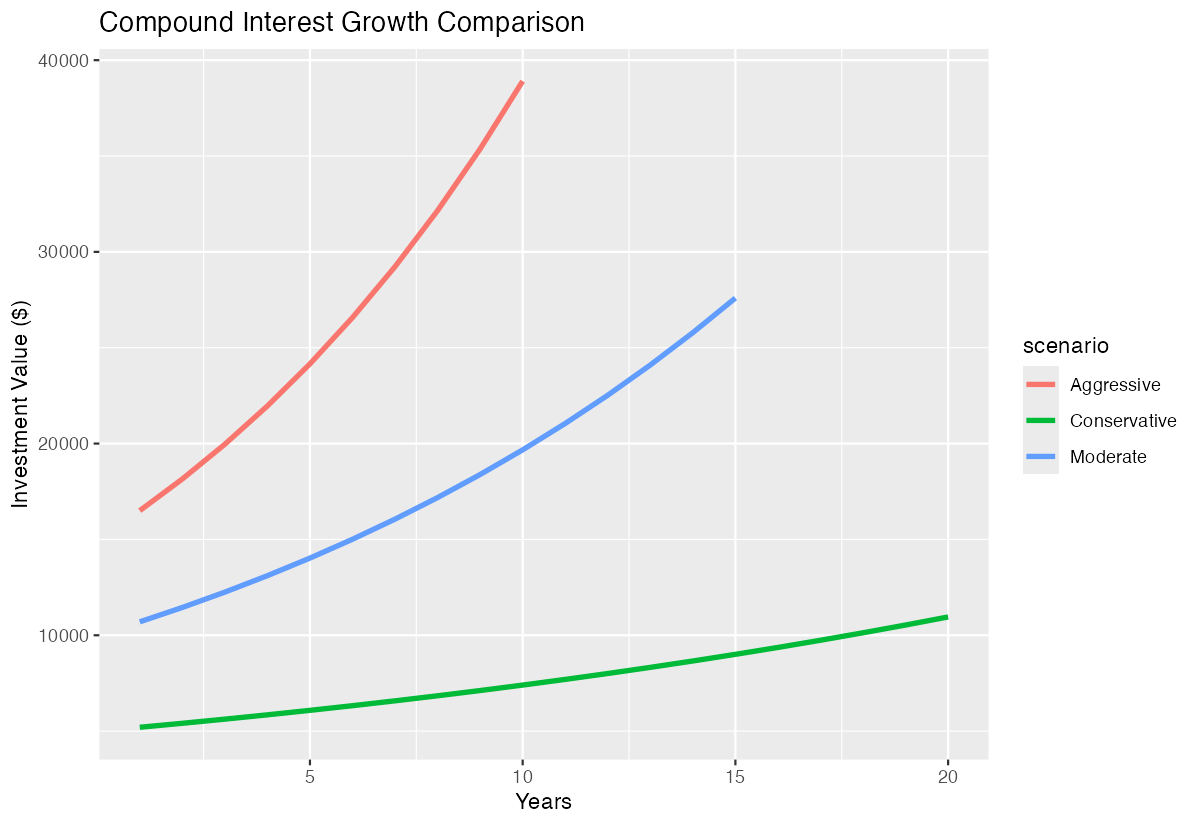
The plot clearly shows how different rates and principals affect long-term growth.
Step 5: Summary Statistics
Finally, we’ll calculate summary statistics for each scenario.
scenario_summary <- yearly_growth |>
  group_by(scenario) |>
  summarise(
    final_value = max(amount),
    total_return = max(interest_earned),
    avg_annual_growth = (max(amount) / principal[1])^(1/max(year_data)) - 1
  )
This provides key metrics to compare the effectiveness of each investment strategy.
Summary
- Use
mutate()with the compound interest formula A = P(1 + r)^t to calculate investment growth - Create multiple scenarios with
tibble()and compare different investment strategies side by side - Expand data with
unnest()androwwise()operations to show year-by-year compound growth - Visualize compound interest trends using
ggplot2to identify optimal investment approaches Generate summary statistics with
group_by()andsummarise()to compare final values and returns across scenarios