How to Calculate Rolling Mean in R
Introduction
Rolling mean (also called moving average) calculates the average of a fixed number of consecutive values in a time series or sequence. It’s essential for smoothing noisy data, identifying trends, and analyzing patterns in financial data, weather measurements, or any sequential observations.
Getting Started
library(tidyverse)
library(palmerpenguins)
Example 1: Basic Rolling Mean
The Problem
We need to calculate a 3-period rolling mean for a simple numeric vector to understand how rolling averages smooth out fluctuations in data.
Step 1: Create Sample Data
Let’s start with a simple numeric vector that has some variation.
# Create sample data with some fluctuation
values <- c(10, 15, 12, 18, 14, 16, 11, 13, 17, 19)
data <- tibble(
  period = 1:10,
  value = values
)
We now have a dataset with 10 periods and corresponding values that fluctuate.
Step 2: Calculate Rolling Mean with zoo Package
We’ll use the rollmean() function from the zoo package for our rolling calculation.
library(zoo)

# Calculate 3-period rolling mean
data <- data |>
  mutate(
    rolling_mean_3 = rollmean(value, k = 3, fill = NA, align = "right")
  )
The rolling mean is calculated using the current and previous 2 values, with NA for insufficient data points.
Step 3: Compare Original vs Smoothed Values
Now let’s examine how the rolling mean smooths our original data.
# View the results
print(data)

# Calculate the difference
data |>
  mutate(difference = value - rolling_mean_3) |>
  select(period, value, rolling_mean_3, difference)
The rolling mean reduces the volatility, showing smoother transitions between periods.
Example 2: Practical Application with Penguin Data
The Problem
We want to analyze penguin body mass trends by calculating rolling averages within each species. This helps identify patterns while reducing the impact of individual measurement variations.
Step 1: Prepare Penguin Data
Let’s filter and arrange the penguin data for our rolling mean analysis.
# Prepare penguin data
penguin_data <- penguins |>
  filter(!is.na(body_mass_g)) |>
  arrange(species, body_mass_g) |>
  group_by(species)
We’ve cleaned the data by removing missing values and grouped by species for separate analysis.
Step 2: Calculate Rolling Means by Species
We’ll calculate both 3-period and 5-period rolling means for each species.
# Calculate rolling means within each species
penguin_rolling <- penguin_data |>
  mutate(
    roll_mean_3 = rollmean(body_mass_g, k = 3, fill = NA, align = "center"),
    roll_mean_5 = rollmean(body_mass_g, k = 5, fill = NA, align = "center")
  ) |>
  ungroup()
Center alignment places the rolling mean at the middle of the window, providing better trend representation.
Step 3: Visualize the Results
Let’s create a plot to compare original values with rolling means.
# Create visualization
penguin_rolling |>
  slice_head(n = 30) |>
  ggplot(aes(x = row_number())) +
  geom_line(aes(y = body_mass_g), alpha = 0.5, color = "gray") +
  geom_line(aes(y = roll_mean_3), color = "blue", size = 1) +
  labs(title = "Penguin Body Mass: Original vs 3-Period Rolling Mean")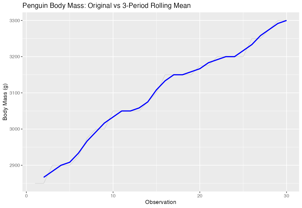
The blue line shows how rolling means smooth out individual variations while preserving the overall trend.
Step 4: Calculate Summary Statistics
Finally, let’s compare the variability between original and smoothed data.
# Compare variability
penguin_rolling |>
  summarise(
    original_sd = sd(body_mass_g, na.rm = TRUE),
    rolling_3_sd = sd(roll_mean_3, na.rm = TRUE),
    rolling_5_sd = sd(roll_mean_5, na.rm = TRUE)
  )
Rolling means show lower standard deviation, confirming their smoothing effect on the data.
Summary
- Rolling means calculate averages over fixed-size moving windows to smooth time series data
- Use
zoo::rollmean()function with parameters for window size (k), fill method, and alignment - Center alignment provides best trend representation, while right alignment is common for forecasting
- Longer rolling windows (higher k values) create smoother trends but may obscure short-term patterns
Rolling means are invaluable for identifying underlying trends in noisy datasets like financial or sensor data