How to Convert Numerical Variable into a Categorical Variable in R
Introduction
Converting numerical variables into categorical variables is a common data preprocessing task that helps create meaningful groups from continuous data. This technique is useful when you want to analyze data by ranges, create ordinal categories, or prepare variables for certain statistical analyses that require categorical inputs.
Getting Started
library(tidyverse)
library(palmerpenguins)
Example 1: Basic Usage
The Problem
We need to convert the continuous body mass variable from the penguins dataset into size categories. This will help us analyze penguins by size groups rather than exact weights.
Step 1: Examine the Data
Let’s first look at the distribution of body mass values.
data(penguins)
penguins |>
  select(species, body_mass_g) |>
  summary()
This shows us the range and distribution of body mass, helping us decide on appropriate category boundaries.
Step 2: Create Categories Using cut()
We’ll divide body mass into three categories: Small, Medium, and Large.
penguins_categorized <- penguins |>
  mutate(size_category = cut(body_mass_g,
                            breaks = 3,
                            labels = c("Small", "Medium", "Large")))
The cut() function automatically creates three equal-width intervals and assigns the specified labels.
Step 3: Verify the Results
Let’s check how many penguins fall into each category.
penguins_categorized |>
  count(size_category) |>
  drop_na()
This shows the distribution of penguins across our newly created size categories.
Example 2: Practical Application
The Problem
We want to create a more nuanced categorization system for penguin flipper length that reflects biological meaningful groups. Instead of equal intervals, we’ll use percentiles to ensure balanced groups for statistical analysis.
Step 1: Calculate Percentiles
First, let’s determine the 25th, 50th, and 75th percentiles for flipper length.
flipper_quantiles <- penguins |>
  summarise(
    q25 = quantile(flipper_length_mm, 0.25, na.rm = TRUE),
    q50 = quantile(flipper_length_mm, 0.50, na.rm = TRUE),
    q75 = quantile(flipper_length_mm, 0.75, na.rm = TRUE)
  )
print(flipper_quantiles)
These percentile values will serve as our category boundaries, ensuring roughly equal sample sizes.
Step 2: Create Custom Categories
Now we’ll use these percentiles as breakpoints for our categories.
penguins_flipper <- penguins |>
  mutate(flipper_category = cut(flipper_length_mm,
                               breaks = c(-Inf, 190, 197, 213, Inf),
                               labels = c("Short", "Medium-Short",
                                        "Medium-Long", "Long")))
Using -Inf and Inf ensures all values are captured, even outliers beyond our calculated range.
Step 3: Cross-Tabulate with Species
Let’s see how flipper categories relate to penguin species.
penguins_flipper |>
  count(species, flipper_category) |>
  drop_na() |>
  pivot_wider(names_from = flipper_category,
              values_from = n,
              values_fill = 0)
This cross-tabulation reveals whether certain species tend to have longer or shorter flippers.
Step 4: Visualize the Categories
Finally, let’s create a visualization to see our categorization in action.
penguins_flipper |>
  drop_na(flipper_category) |>
  ggplot(aes(x = flipper_category, fill = species)) +
  geom_bar(position = "dodge") +
  labs(title = "Penguin Count by Flipper Category and Species")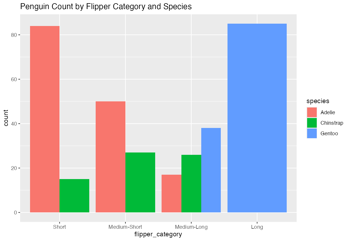
This bar chart clearly shows the relationship between our created categories and the original species variable.
Summary
- Use
cut()withbreaksparameter to create equal-width intervals from numerical data - Specify custom
labelsto make categories more interpretable than default ranges - Calculate percentiles first when you need balanced group sizes rather than equal intervals
- Use
-InfandInfas boundary values to capture all possible data points including outliers Always verify your categorization with
count()and cross-tabulation to ensure meaningful groups