Effect of centering and scaling data in R
Introduction
Data scaling and centering are essential preprocessing steps in data analysis and machine learning. These transformations help normalize variables with different units and scales, making them comparable and improving the performance of many algorithms. We’ll explore how to visualize and apply these transformations using R and the Palmer penguins dataset.
Loading Required Libraries
Let’s start by loading the necessary packages for our analysis.
library(tidyverse)
library(palmerpenguins)
library(ggridges)
theme_set(theme_bw(16))
Preparing the Data
First, we’ll prepare our dataset by removing missing values and selecting only the numeric variables.
df <- penguins |>
  drop_na() |>
  select(-year) |>
  select(where(is.numeric))
Let’s examine the first few rows to understand our data structure.
df |> head()Our dataset now contains four numeric variables: bill length, bill depth, flipper length, and body mass, all measured on different scales.
Visualizing Raw Data Distributions
Before applying any transformations, let’s visualize how our variables are distributed using boxplots.
df |>
  mutate(row_id = row_number()) |>
  pivot_longer(-row_id, names_to = "feature", values_to = "value") |>
  ggplot(aes(x = feature, y = value, color = feature)) +
  geom_boxplot(outlier.shape = NA) +
  geom_jitter(width = 0.1) +
  labs(title = "Raw Penguin Measurements on Different Scales",
       x = "Feature", y = "Value") +
  theme(legend.position = "none")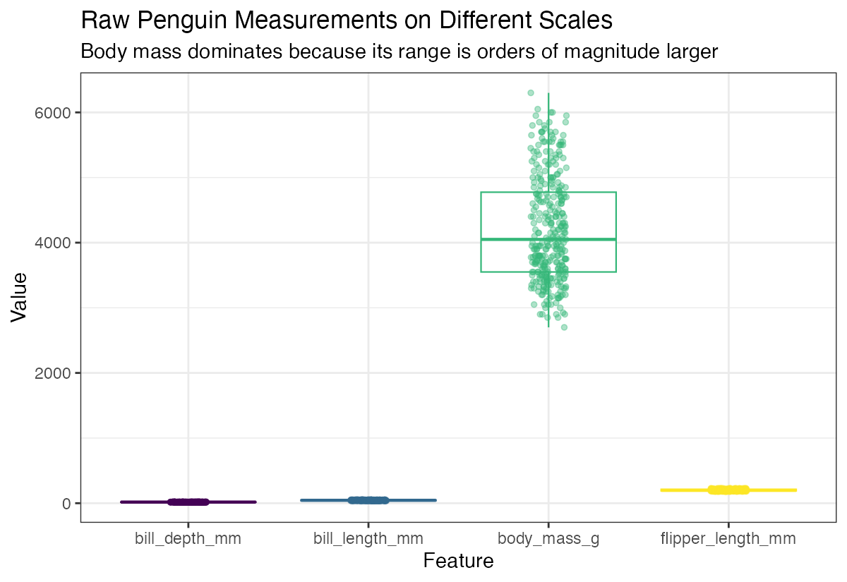
Notice how the variables have very different ranges - body mass is in thousands while bill measurements are in tens. This makes direct comparison difficult.
Using Ridge Plots for Better Comparison
Ridge plots provide a clearer view of each variable’s distribution shape.
df |>
  mutate(row_id = row_number()) |>
  pivot_longer(-row_id, names_to = "feature", values_to = "value") |>
  ggplot(aes(y = feature, x = value, fill = feature)) +
  geom_density_ridges2() +
  theme(legend.position = "none")
The different scales make it challenging to compare distribution shapes across variables.
Scaling and Centering Data
Now let’s apply both centering (subtracting the mean) and scaling (dividing by standard deviation) to standardize our variables.
df_scaled <- df |>
  scale(center = TRUE, scale = TRUE)
Let’s examine the transformed data.
df_scaled |> head()The scaled data now has a mean of 0 and standard deviation of 1 for each variable, making them directly comparable.
Visualizing Scaled Data
Let’s see how the scaling transformation affects our distributions.
df_scaled |>
  as.data.frame() |>
  mutate(row_id = row_number()) |>
  pivot_longer(-row_id, names_to = "feature", values_to = "value") |>
  ggplot(aes(y = feature, x = value, fill = feature)) +
  geom_density_ridges2() +
  labs(title = "After Centering and Scaling (mean 0, sd 1)",
       x = "Standardized value", y = "Feature") +
  theme(legend.position = "none")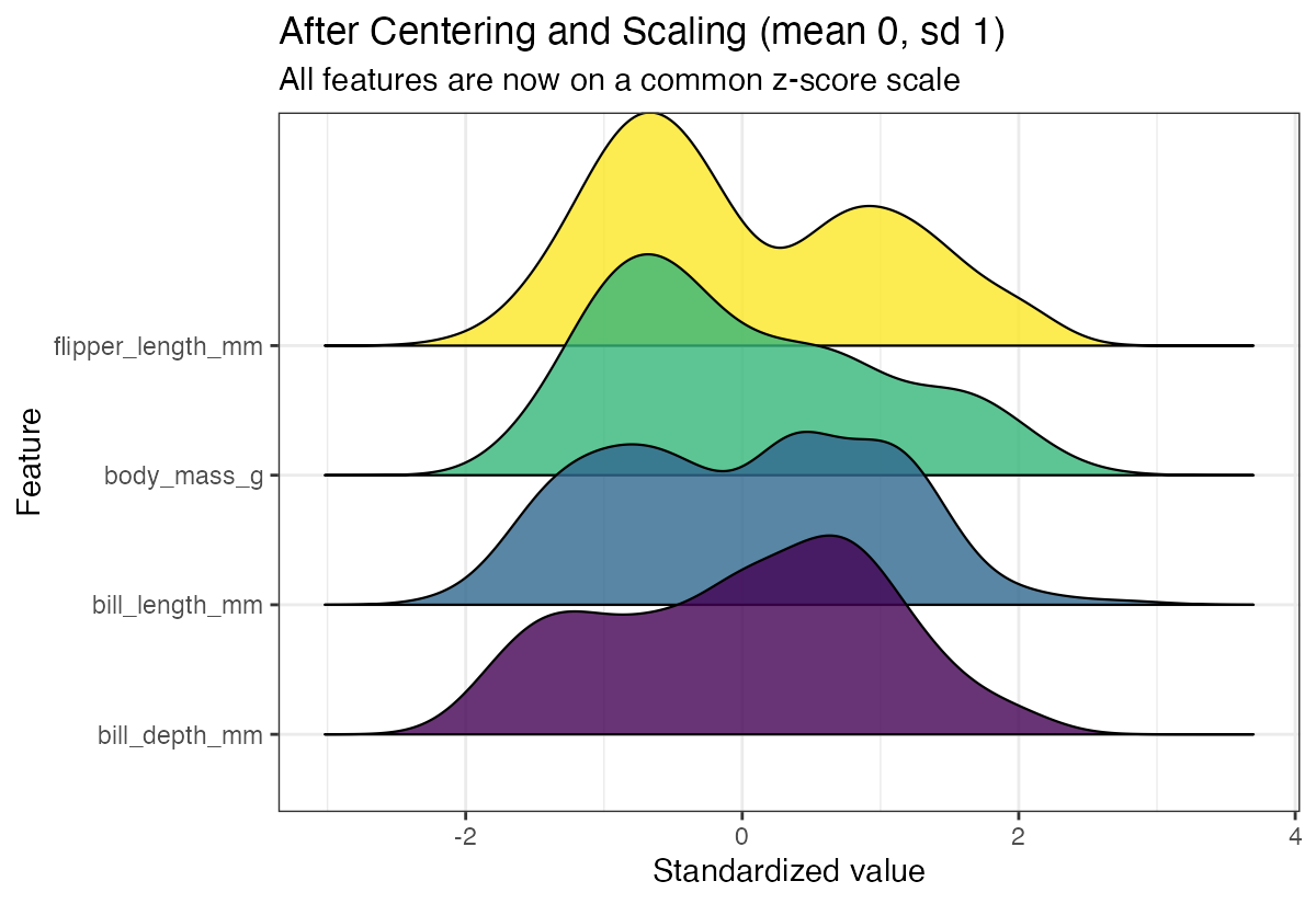
Now all variables are on the same scale, making it easy to compare their distribution shapes and identify which variables have the most variability.
Centering Only (Without Scaling)
Sometimes you might want to center data without scaling. This shifts distributions to have a mean of 0 but preserves the original variance.
df_centered <- df |>
  scale(center = TRUE, scale = FALSE)
Let’s examine the centered-only data.
df_centered |> head()Visualizing Centered Data
Here’s how centering without scaling affects our distributions.
df_centered |>
  as.data.frame() |>
  mutate(row_id = row_number()) |>
  pivot_longer(-row_id, names_to = "feature", values_to = "value") |>
  ggplot(aes(y = feature, x = value, fill = feature)) +
  geom_density_ridges2() +
  labs(title = "After Centering Only (mean 0, original spreads)",
       x = "Centered value", y = "Feature") +
  theme(legend.position = "none")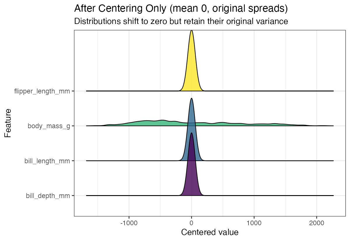
The distributions maintain their original spreads but are now centered around zero, which can be useful for certain analyses while preserving the relative scale differences.
Summary
Data scaling and centering are powerful preprocessing techniques that make variables comparable and improve analysis quality. Use full scaling (center = TRUE, scale = TRUE) when you want all variables on the same scale, such as for machine learning algorithms. Use centering only (center = TRUE, scale = FALSE) when you want to preserve relative scale differences but center distributions around zero. Visual exploration with ridge plots helps you understand the impact of these transformations on your data.