How to calculate compound interest in R
Introduction
Compound interest is one of the most powerful concepts in finance - it’s the process where your investment earns returns not just on the initial amount, but also on all previously earned interest. In this tutorial, we’ll use R and the tidyverse to calculate, analyze, and visualize compound interest scenarios to help you understand how investments grow over time.
Setting Up Our Analysis
First, let’s load the required packages and set up our basic parameters for compound interest calculations.
library(tidyverse)
library(scales)
library(gt)
theme_set(theme_bw(16))
Now we’ll define our initial investment scenario with clear, realistic parameters.
principal <- 1000    # Starting amount
years <- 10          # Time period in years
rate <- 0.05         # Interest rate (5%)
These variables represent a $1,000 investment over 10 years at 5% annual interest - a common scenario for understanding compound growth.
Creating the Basic Data Structure
Let’s start by creating a tibble with years from 0 to 10 to track our investment over time.
tibble(year = 0:years)This creates our foundation - a simple table with one column showing each year of our investment period.
Calculating Compound Interest
Now we’ll add the compound interest calculation using the standard formula: A = P(1 + r)^t.
compound_data <- tibble(year = 0:years) |>
  mutate(amount = principal * (1 + rate) ^ year)
The amount column now shows how our $1,000 grows each year, with interest compounding annually.
Adding Interest Earned
Let’s enhance our analysis by calculating how much interest we’ve earned above our initial investment.
compound_data <- tibble(year = 0:years) |>
  mutate(
    amount = principal * (1 + rate) ^ year,
    interest_earned = amount - principal
  )

print(compound_data)
The interest_earned column shows the cumulative interest gained, making it easy to see the power of compounding over time.
Visualizing Single Investment Growth
A line chart helps visualize how compound interest accelerates over time.
compound_data |>
  ggplot(aes(x = year, y = amount)) +
  geom_line(color = "blue", linewidth = 1) +
  geom_point(color = "red", size = 2) +
  labs(
    title = paste("Compound Interest Over", years, "Years"),
    x = "Year",
    y = "Investment Value",
    subtitle = paste("Starting with $", scales::comma(principal), "at", rate * 100, "% annual interest")
  ) +
  scale_y_continuous(labels = label_currency())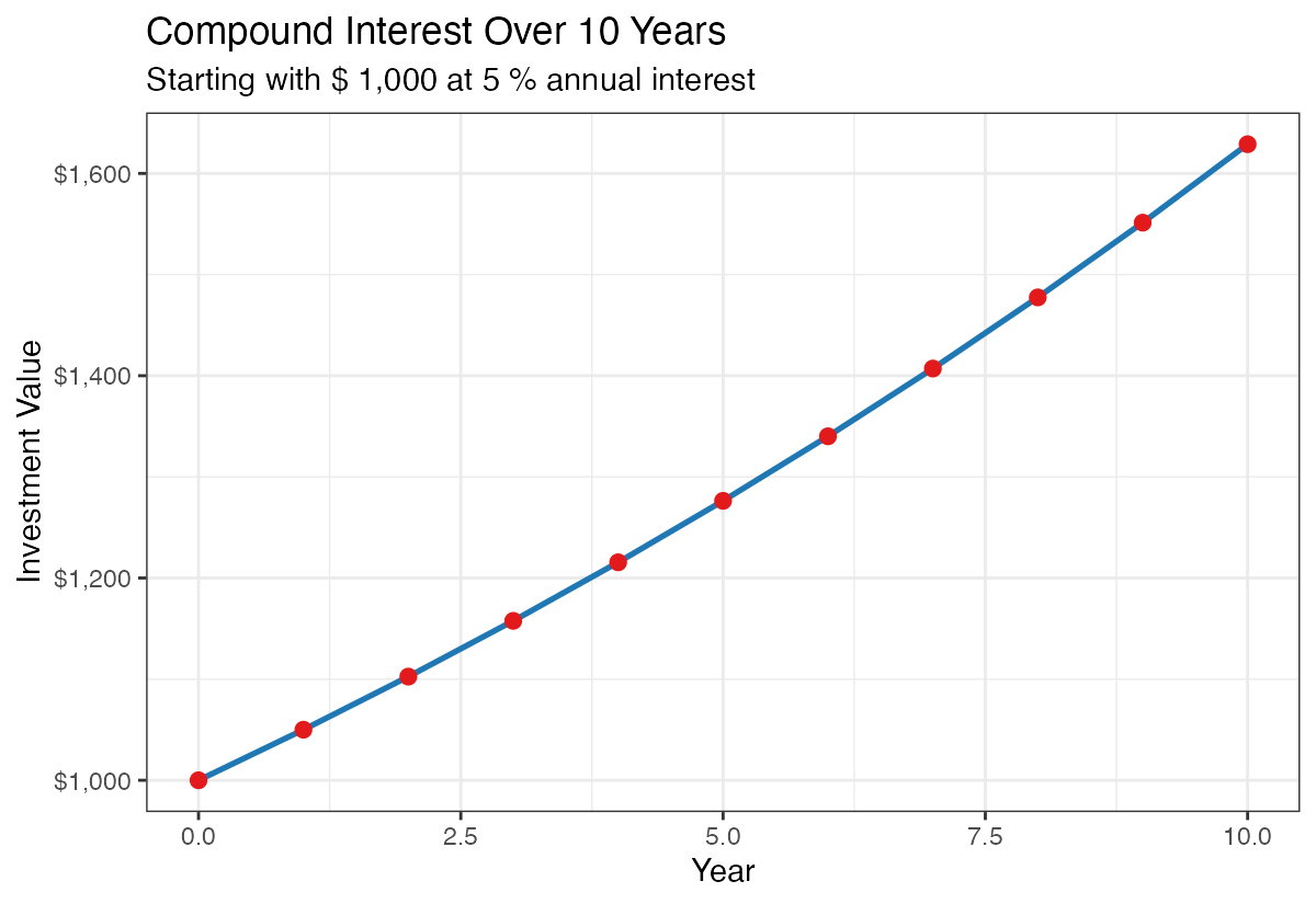
This visualization clearly shows the exponential nature of compound growth - notice how the curve gets steeper in later years.
Scaling Up: Larger Investment Example
Let’s see how compound interest works with a larger investment amount like $500,000.
principal_large <- 500000
years <- 10
rate <- 0.05

large_investment <- tibble(year = 0:years) |>
  mutate(
    amount = principal_large * (1 + rate) ^ year,
    interest_earned = amount - principal_large
  )
With a larger principal, the absolute dollar growth becomes much more dramatic, though the percentage growth remains the same.
Visualizing the Larger Investment
large_investment |>
  ggplot(aes(x = year, y = amount)) +
  geom_line(color = "green4", linewidth = 1) +
  geom_point(color = "red", size = 2) +
  labs(
    title = "Compound Interest: $500K Investment",
    x = "Year",
    y = "Investment Value",
    subtitle = paste("Growth at", rate * 100, "% annual interest")
  ) +
  scale_y_continuous(labels = label_currency())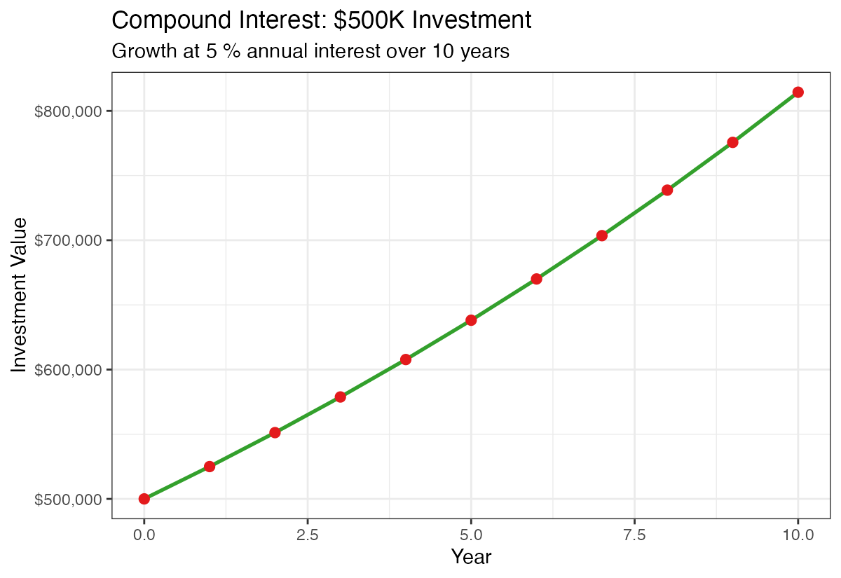
The same 5% rate now generates tens of thousands in additional value each year due to the larger base amount.
Comparing Multiple Interest Rates
Real investments have varying returns, so let’s compare different interest rate scenarios.
rates <- seq(0.04, 0.10, by = 0.02)  # 4%, 6%, 8%, 10%
principal <- 500000
years <- 10
These rates represent a realistic range from conservative (4%) to optimistic (10%) annual returns.
Creating Multi-Rate Comparison Data
We’ll use expand_grid() to create all combinations of years and interest rates.
multi_rate_data <- expand_grid(year = 0:years, rate = rates) |>
  mutate(
    amount = principal * (1 + rate) ^ year,
    interest_earned = amount - principal
  )
This creates a comprehensive dataset showing how the same investment performs under different interest rate scenarios.
Visualizing Rate Comparisons
multi_rate_data |>
  ggplot(aes(x = year, y = amount, color = factor(rate))) +
  geom_line(linewidth = 1) +
  geom_point(size = 2) +
  labs(
    title = "Compound Interest: Impact of Different Rates",
    x = "Year",
    y = "Investment Value",
    color = "Interest Rate",
    subtitle = paste("Starting investment: $", scales::comma(principal))
  ) +
  scale_y_continuous(labels = label_currency())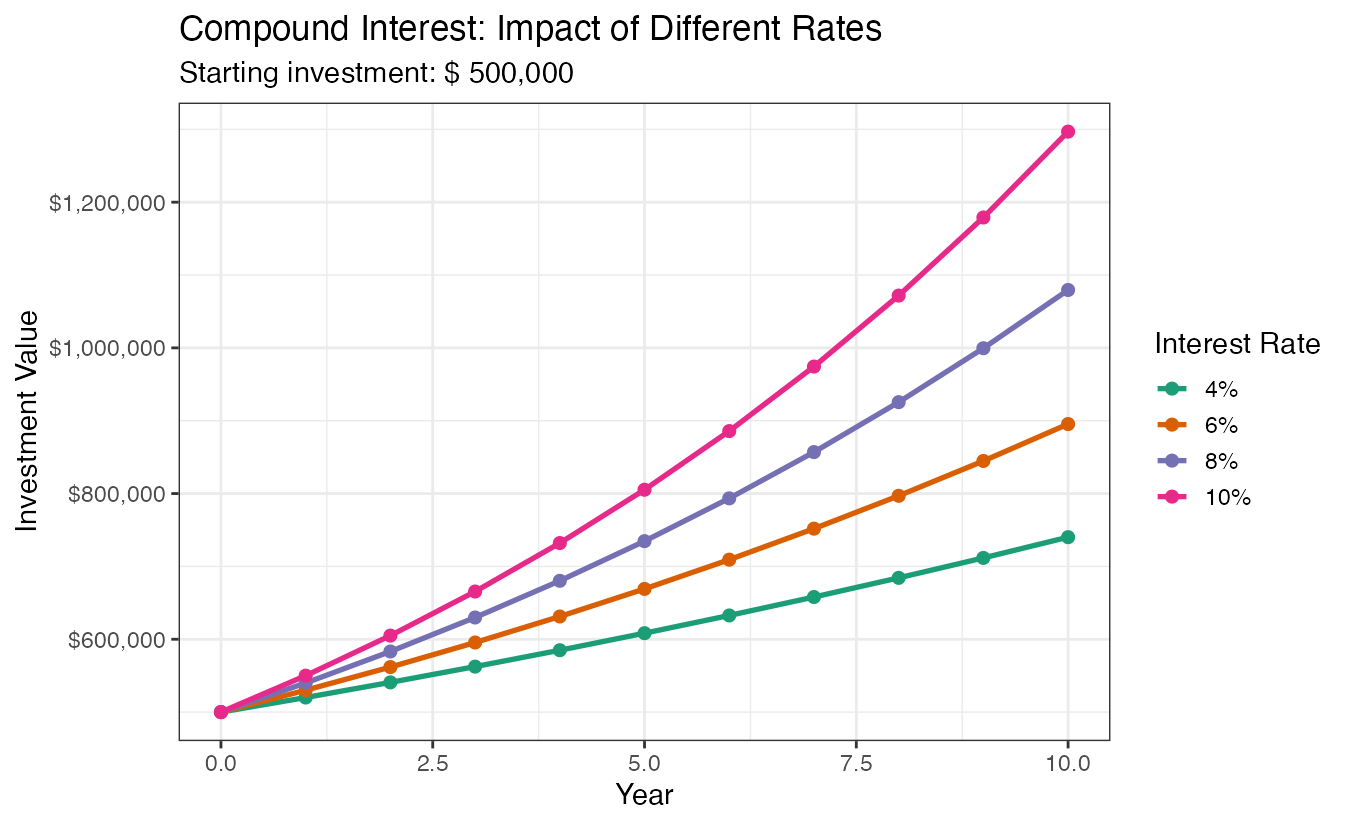
This comparison dramatically shows how even small differences in interest rates (like 2%) can result in huge differences in final value over time.
Creating a Comparison Table
For precise comparisons, let’s create a formatted table showing values at each rate.
multi_rate_data |>
  select(year, rate, amount) |>
  pivot_wider(
    names_from = rate,
    values_from = amount,
    names_glue = "{rate*100}% Rate"
  ) |>
  gt() |>
  fmt_currency(columns = -year)
This table format makes it easy to compare exact dollar amounts across different scenarios and time periods.
Summary
Compound interest calculations in R demonstrate the powerful concept of exponential growth over time. Using tidyverse tools like tibble(), mutate(), and expand_grid(), we can easily model different investment scenarios and visualize how small changes in interest rates or time periods create dramatic differences in outcomes. The key insight is that compound interest rewards both higher rates and longer time horizons, with the effects becoming more pronounced as investments mature. These R techniques can be applied to any financial planning scenario, from retirement savings to loan calculations.