How to calculate Pearson correlation in R
Introduction
Data scaling and centering are fundamental preprocessing steps in data analysis and machine learning. Scaling transforms variables to have similar ranges, while centering adjusts variables to have a mean of zero. These transformations are essential when working with variables of different units or magnitudes, ensuring that no single variable dominates analyses due to its scale.
Setup and Data Preparation
Let’s start by loading the necessary libraries and preparing our dataset.
library(tidyverse)
library(palmerpenguins)
theme_set(theme_bw(16))
We’ll use the Palmer Penguins dataset, selecting only the numeric variables for our scaling demonstration.
df <- penguins |>
  drop_na() |>
  select(-year) |>
  select(where(is.numeric))
Let’s examine our cleaned dataset structure:
df |> head()This gives us four numeric variables: bill length, bill depth, flipper length, and body mass, all measured in different units and scales.
Understanding Variable Scales
Before scaling, let’s visualize how our variables differ in their ranges and distributions.
df |>
  mutate(row_id = row_number()) |>
  pivot_longer(-row_id, names_to = "feature", values_to = "value") |>
  ggplot(aes(x = feature, y = value, color = feature)) +
  geom_boxplot(outlier.shape = NA) +
  geom_jitter(width = 0.1) +
  scale_y_log10() +
  theme(legend.position = "none")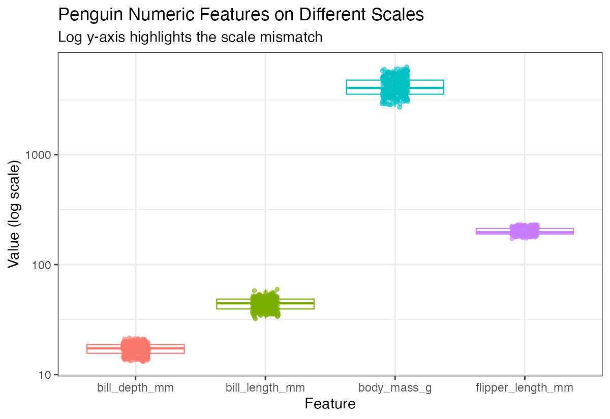
Notice how body mass ranges in thousands while bill measurements are in tens - this dramatic difference in scales can problematic for many analyses.
Standardization (Z-score Scaling)
Standardization transforms variables to have a mean of 0 and standard deviation of 1. This is the default behavior of the scale() function.
df_scaled <- df |> scale()
df_scaled |> head()
Let’s visualize the scaled data to see how the distributions now compare:
df_scaled |>
  as.data.frame() |>
  mutate(row_id = row_number()) |>
  pivot_longer(-row_id, names_to = "feature", values_to = "value") |>
  ggplot(aes(x = feature, y = value, color = feature)) +
  geom_boxplot(outlier.shape = NA) +
  geom_jitter(width = 0.1) +
  theme(legend.position = "none")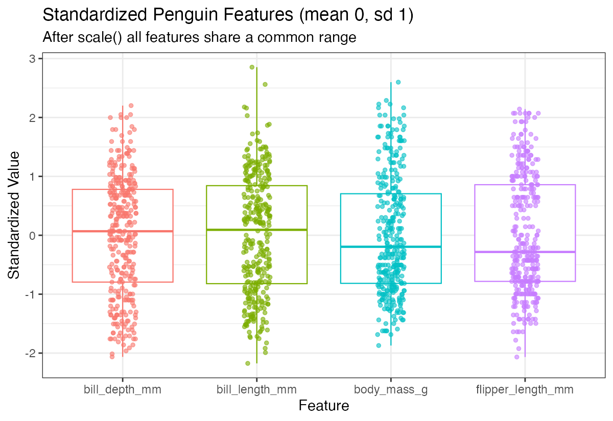
Now all variables have similar scales, making them directly comparable. The standardized variables are centered around 0 with similar spreads.
Centering Only
Sometimes you may want to center variables (mean = 0) without scaling them. Use the center and scale parameters explicitly:
df_centered <- df |>
  scale(center = TRUE, scale = FALSE)
df_centered |> head()
Centering alone shifts the distribution but preserves the original scale relationships between variables.
Verifying Transformations
Let’s confirm our scaling worked by checking the means of our standardized data:
colMeans(df_scaled)All means should be essentially zero (within floating-point precision). Now let’s check the covariance matrix:
cov(df_scaled)For standardized data, the covariance matrix equals the correlation matrix, since standardization makes the variance of each variable equal to 1.
Working with Correlation Matrices
The correlation matrix shows the linear relationships between variables:
cor(df_scaled)You can also calculate correlations between subsets of variables:
cor(df_scaled[,1:2], df_scaled[,3:4])This shows correlations between the first two variables (bill measurements) and the last two (flipper length and body mass).
Matrix Multiplication Approach
Understanding that correlation can be computed through matrix multiplication helps grasp the mathematical foundation:
n <- nrow(df_scaled)
(t(df_scaled) %*% df_scaled) / (n - 1)
This manual calculation produces the same result as the cor() function, demonstrating how correlation matrices are computed mathematically.
Let’s verify this matches the built-in function:
cor(df_scaled)Both approaches yield identical results, confirming our understanding of the underlying mathematics.
Summary
Data scaling and centering are crucial preprocessing steps that ensure variables contribute equally to analyses. Standardization (z-score scaling) creates variables with mean 0 and standard deviation 1, while centering only adjusts the mean. The scale() function in R provides flexible options for these transformations, and understanding the relationship between scaled data and correlation matrices helps build intuition for multivariate analyses. Always visualize your data before and after scaling to ensure the transformations achieve your analytical goals.