How to calculate z-scores in R
Introduction
A z-score is a statistical measure that describes how far a data point is from the mean of a dataset, expressed in terms of standard deviations. Z-scores are essential for standardizing data across different scales, identifying outliers, and comparing values from different distributions. In this tutorial, we’ll learn how to calculate z-scores in R using both manual calculations and built-in functions.
Understanding Z-Scores
The z-score formula is: z = (X - μ) / σ
Where: - X is the individual data point - μ (mu) is the mean of the dataset
- σ (sigma) is the standard deviation of the dataset
Interpreting z-scores: - A z-score of 0 means the data point equals the mean - Positive z-scores indicate values above the mean - Negative z-scores indicate values below the mean - The magnitude shows how many standard deviations away from the mean
For example, if test scores have a mean of 70 and standard deviation of 10, a score of 85 has a z-score of (85-70)/10 = 1.5, meaning it’s 1.5 standard deviations above average.
Setting Up Our Data
First, let’s load the necessary packages and examine our dataset. We’ll use the Palmer penguins data to demonstrate z-score calculations.
library(tidyverse)
library(palmerpenguins)
Let’s explore the penguins dataset and select two numeric variables for our z-score analysis.
penguins |>
  glimpse()
We can see various measurements for different penguin species. Let’s focus on bill depth and body mass for our z-score calculations.
Preparing the Data
We need to clean our data by removing missing values and selecting our variables of interest.
df <- penguins |>
  drop_na() |>
  select(bill_depth_mm, body_mass_g)
Now let’s examine the basic statistics of our selected variables.
df |>
  head()
df |>
summary()This shows us the distribution of our variables. Notice the different scales - bill depth is measured in millimeters (around 15-20) while body mass is in grams (around 3000-6000).
Manual Z-Score Calculation
Let’s calculate z-scores manually using the formula. This helps us understand exactly what’s happening mathematically.
df <- df |>
  mutate(
    bill_depth_zscore_manual = (bill_depth_mm - mean(bill_depth_mm)) / sd(bill_depth_mm),
    body_mass_zscore_manual = (body_mass_g - mean(body_mass_g)) / sd(body_mass_g)
  )
df |>
head()Now our data includes the original measurements and their corresponding z-scores. Notice how the z-scores are on a similar scale regardless of the original units.
Using R’s Built-in Scale Function
R provides a convenient scale() function that calculates z-scores automatically. Let’s use it and compare with our manual calculation.
df <- df |>
  mutate(
    bill_depth_zscore = c(scale(bill_depth_mm)),
    body_mass_zscore = c(scale(body_mass_g))
  )
The c() function converts the matrix output of scale() into a vector that works well with mutate().
Let’s verify our calculations by examining the summary statistics of our z-scores.
df |>
  select(contains("zscore")) |>
  summary()
Notice that z-scores have a mean of approximately 0 and standard deviation of 1. This is the key property of standardized scores.
Verifying Our Calculations
Let’s confirm that both methods produce identical results.
all.equal(df$bill_depth_zscore_manual, df$bill_depth_zscore)This should return TRUE, confirming our manual calculation matches R’s built-in function.
Visualizing Z-Score Transformations
Let’s create visualizations to understand how z-scores transform our data. First, let’s see the relationship between original values and their z-scores.
df |>
  ggplot(aes(x = bill_depth_mm, y = bill_depth_zscore)) +
  geom_point(alpha = 0.7) +
  labs(
    title = "Original Bill Depth vs Z-Score",
    x = "Bill Depth (mm)",
    y = "Z-Score"
  )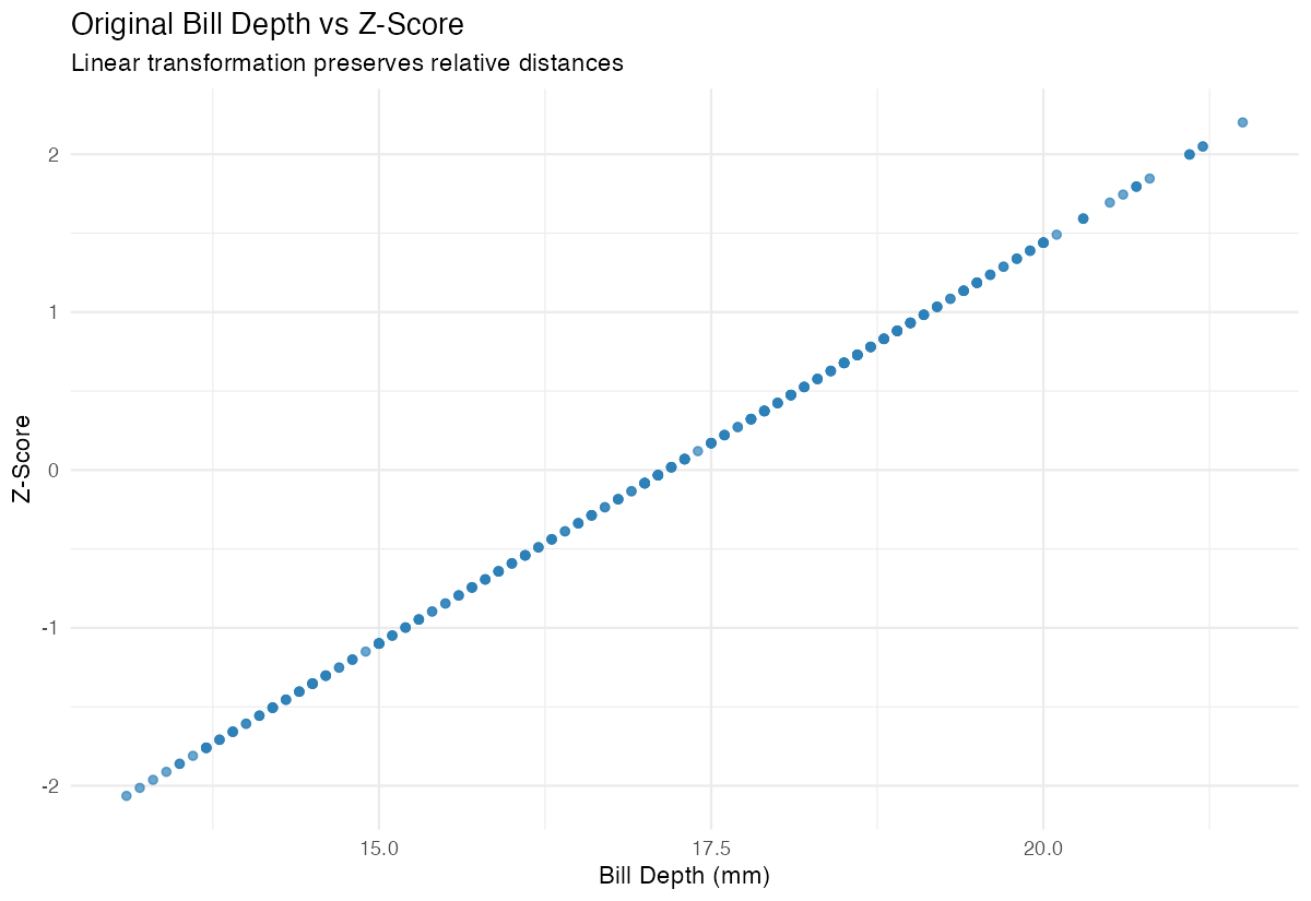
This plot shows the linear relationship between original values and z-scores. The transformation preserves the relative relationships while changing the scale.
Let’s also verify that both calculation methods produce identical results visually.
df |>
  ggplot(aes(x = bill_depth_zscore_manual, y = bill_depth_zscore)) +
  geom_point(alpha = 0.7) +
  geom_abline(intercept = 0, slope = 1, color = "red", linetype = "dashed") +
  labs(
    title = "Manual vs Built-in Z-Score Calculation",
    x = "Manual Z-Score",
    y = "Built-in Z-Score"
  )
The points should fall exactly on the diagonal line, confirming both methods are equivalent.
Comparing Distributions
One powerful use of z-scores is comparing values across different distributions. Let’s create a comparison plot.
df |>
  select(bill_depth_zscore, body_mass_zscore) |>
  pivot_longer(everything(), names_to = "variable", values_to = "zscore") |>
  ggplot(aes(x = zscore, fill = variable)) +
  geom_histogram(alpha = 0.7, bins = 30) +
  facet_wrap(~variable) +
  labs(
    title = "Distribution of Z-Scores",
    x = "Z-Score",
    y = "Count"
  )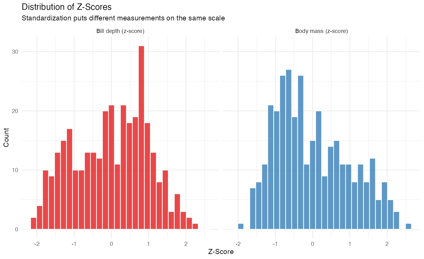
Both distributions are now on the same standardized scale, making them directly comparable despite their very different original units.
Summary
Z-scores are powerful tools for standardizing data and making comparisons across different scales. In R, you can calculate them manually using the formula (x - mean(x)) / sd(x) or use the convenient scale() function. Z-scores transform any distribution to have a mean of 0 and standard deviation of 1, while preserving the original relationships between data points. This makes them invaluable for data analysis, outlier detection, and comparing measurements across different variables or datasets.