How to Pearson correlation in R
Introduction
Pearson correlation measures the linear relationship between two continuous variables, producing a value between -1 and 1. Use it when you want to understand how strongly two numeric variables move together in a linear fashion.
Getting Started
library(tidyverse)
library(palmerpenguins)
Example 1: Basic Usage
The Problem
We want to examine if there’s a relationship between penguin flipper length and body mass. This will help us understand basic penguin anatomy relationships.
Step 1: Load and examine the data
First, let’s look at our penguin dataset structure.
data(penguins)
penguins |>
  select(flipper_length_mm, body_mass_g) |>
  head()
This shows us the first few rows of our two variables of interest.
Step 2: Calculate basic correlation
Now we’ll compute the Pearson correlation coefficient.
correlation <- cor(penguins$flipper_length_mm,
                   penguins$body_mass_g,
                   use = "complete.obs")
print(correlation)
The use = "complete.obs" parameter handles missing values by excluding incomplete pairs.
Step 3: Create a visualization
Let’s visualize this relationship with a scatter plot.
penguins |>
  filter(!is.na(flipper_length_mm), !is.na(body_mass_g)) |>
  ggplot(aes(x = flipper_length_mm, y = body_mass_g)) +
  geom_point(alpha = 0.7) +
  geom_smooth(method = "lm") +
  labs(title = "Penguin Flipper Length vs Body Mass")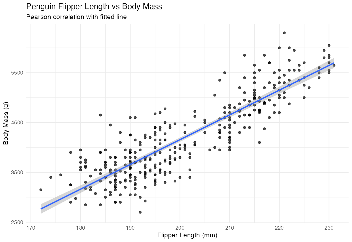
This plot confirms the strong positive correlation we calculated numerically.
Example 2: Practical Application
The Problem
A marine biologist wants to analyze correlations between multiple penguin measurements across different species. They need to test statistical significance and handle different groups properly.
Step 1: Perform correlation test
We’ll use cor.test() to get statistical significance along with the correlation.
correlation_test <- cor.test(penguins$flipper_length_mm,
                            penguins$body_mass_g,
                            method = "pearson")
print(correlation_test)
This provides the correlation coefficient, confidence interval, and p-value for hypothesis testing.
Step 2: Calculate correlation matrix
Let’s examine correlations between multiple numeric variables simultaneously.
numeric_vars <- penguins |>
  select(bill_length_mm, bill_depth_mm,
         flipper_length_mm, body_mass_g)

correlation_matrix <- cor(numeric_vars, use = "complete.obs")
round(correlation_matrix, 3)
The correlation matrix shows relationships between all pairs of variables in a single table.
Step 3: Group by species
Now we’ll calculate correlations separately for each penguin species.
species_correlations <- penguins |>
  group_by(species) |>
  summarise(
    correlation = cor(flipper_length_mm, body_mass_g,
                     use = "complete.obs"),
    .groups = "drop"
  )
print(species_correlations)
This reveals how the flipper-mass relationship varies across different penguin species.
Step 4: Visualize by groups
Finally, let’s create a grouped visualization to see these relationships.
penguins |>
  filter(!is.na(flipper_length_mm), !is.na(body_mass_g), !is.na(species)) |>
  ggplot(aes(x = flipper_length_mm, y = body_mass_g,
             color = species)) +
  geom_point(alpha = 0.7) +
  geom_smooth(method = "lm", se = FALSE) +
  labs(title = "Flipper Length vs Body Mass by Species")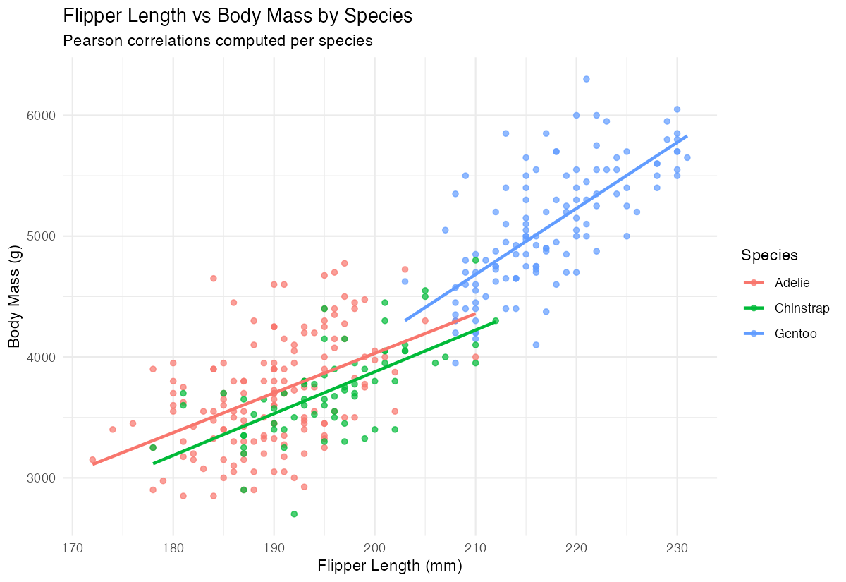
The different colored trend lines show how correlation strength varies between Adelie, Chinstrap, and Gentoo penguins.
Summary
• Use cor() for simple correlation coefficients and cor.test() when you need statistical significance testing • Always include use = "complete.obs" to properly handle missing values in your data • Correlation matrices with cor() efficiently compare multiple variables simultaneously
• Group-wise correlations using group_by() reveal how relationships differ across categories • Scatter plots with trend lines provide essential visual confirmation of your correlation calculations —