How to perform a t-test in R
Introduction
A t-test is one of the most commonly used statistical tests for determining if there is a significant difference between the means of two groups. It’s particularly useful when comparing things like heights between men and women, test scores before and after an intervention, or measurements between treatment and control groups.
Setting Up Your Environment
First, let’s load the necessary packages for our analysis and visualization:
library(palmerpenguins)
library(tidyverse)
library(broom)
theme_set(theme_bw(16))
We’ll use palmerpenguins for real-world data, tidyverse for data manipulation and plotting, and broom for cleaning up statistical output.
Creating Sample Data
Let’s start by creating two groups with simulated data to understand how t-tests work:
set.seed(123)
x <- rnorm(n = 15, mean = 10, sd = 1)
y <- rnorm(n = 15, mean = 15, sd = 1)
Here we’re generating two groups of 15 observations each, where group x has a mean of 10 and group y has a mean of 15, both with standard deviation of 1.
Let’s check the actual means of our generated data:
mean(x)
mean(y)
The means should be close to 10 and 15 respectively, though they won’t be exactly those values due to random sampling.
Performing a Basic T-Test
Now let’s perform our first t-test to compare these two groups:
t_test_res <- t.test(x, y)
t_test_res
This gives us the complete t-test output including the t-statistic, degrees of freedom, p-value, and confidence interval.
Extracting Specific Results
You can extract specific components from the t-test results:
t_test_res$p.value
t_test_res$statistic
The p-value tells us the probability of observing this difference (or larger) if there truly was no difference between groups. The statistic is the calculated t-value.
For a cleaner output format, we can use the broom package:
t_test_res |> broom::tidy()This creates a tidy data frame with all the key results, making it easier to work with programmatically.
Visualizing the Data
Let’s create a visualization to see the difference between our groups:
tibble(
  group = c(rep("g1", 15), rep("g2", 15)),
  data = c(x, y)
) |>
  ggplot(aes(x = group, y = data, fill = group)) +
  geom_boxplot(outlier.shape = NA) +
  geom_jitter(width = 0.1) +
  theme(legend.position = "none") +
  labs(title = "Two groups with a clear difference in mean",
x = "Group", y = "Value")![]()
This plot clearly shows the separation between the two groups, which corresponds to our highly significant t-test result.
Example with No Significant Difference
Let’s create another example where the groups have the same mean but different variances:
set.seed(123)
x <- rnorm(n = 15, mean = 10, sd = 1)
y <- rnorm(n = 15, mean = 10, sd = 2)

t_test_res <- t.test(x, y)
t_test_res |> broom::tidy()
Since both groups have the same underlying mean (10), we expect a non-significant result (p-value > 0.05).
Let’s visualize this comparison:
tibble(
  group = c(rep("g1", 15), rep("g2", 15)),
  data = c(x, y)
) |>
  ggplot(aes(x = group, y = data, fill = group)) +
  geom_boxplot(outlier.shape = NA) +
  geom_jitter(width = 0.1) +
  theme(legend.position = "none") +
  labs(title = "Two groups with NO clear difference in mean",
       x = "Group", y = "Value")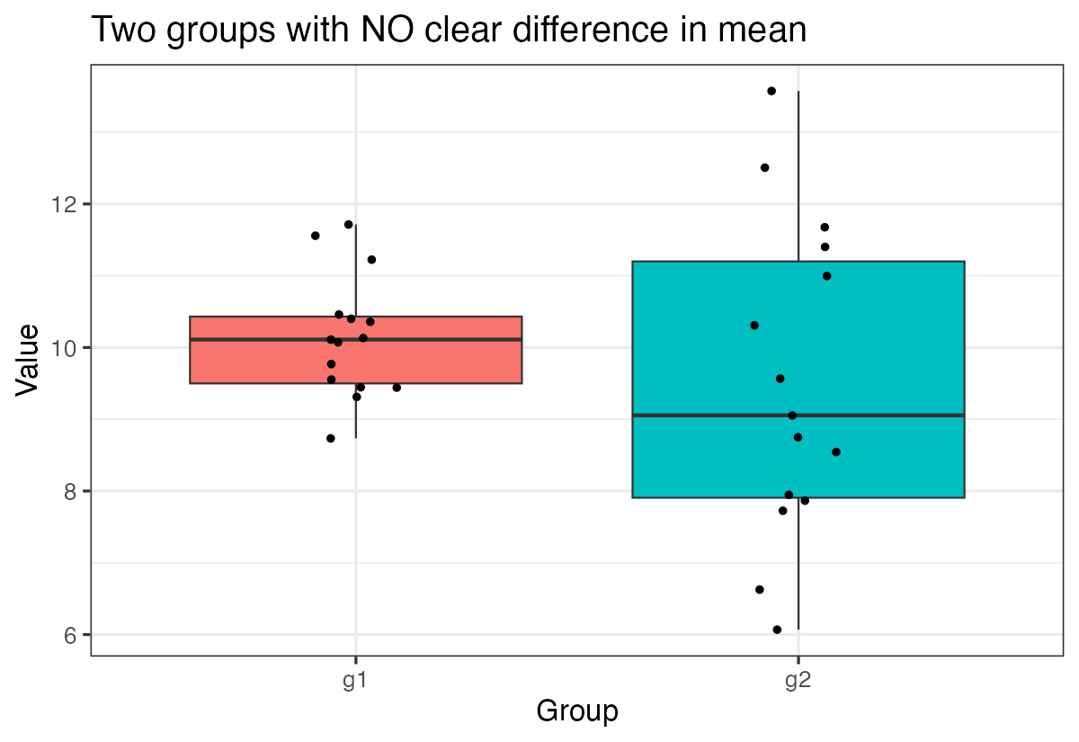
Notice how the boxplots overlap much more, reflecting the lack of significant difference between groups.
Using Real-World Data
Now let’s work with real data from the Palmer Penguins dataset. We’ll compare bill length between male and female penguins:
set.seed(1234)
df <- penguins |>
  drop_na() |>
  select(sex, bill_length_mm) |>
  group_by(sex) |>
  slice_sample(n = 15) |>
  ungroup()
We’re taking a random sample of 15 penguins from each sex group to create a smaller dataset for comparison.
Let’s visualize this real-world comparison:
df |>
  ggplot(aes(x = sex, y = bill_length_mm, fill = sex)) +
  geom_boxplot(outlier.shape = NA) +
  geom_jitter(width = 0.1) +
  theme(legend.position = "none") +
  labs(title = "Penguin Bill Length by Sex (n = 15 per group)",
       x = "Sex", y = "Bill Length (mm)")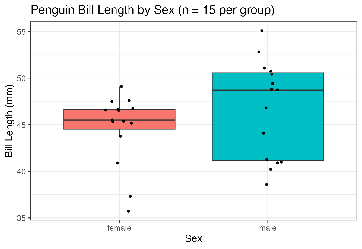
Now let’s perform the t-test on this real data using a more advanced approach:
df |>
  summarize(t_test = list(t.test(bill_length_mm ~ sex))) |>
  mutate(ttest = map(t_test, tidy)) |>
  unnest(ttest)
This approach uses the formula notation (bill_length_mm ~ sex) and demonstrates how to perform t-tests within a data analysis pipeline.
The Impact of Sample Size
Let’s see what happens when we use the full dataset instead of just 15 samples per group:
penguins |>
  drop_na() |>
  ggplot(aes(x = sex, y = bill_length_mm, fill = sex)) +
  geom_boxplot(outlier.shape = NA) +
  geom_jitter(width = 0.1) +
  theme(legend.position = "none") +
  labs(title = "Penguin Bill Length by Sex (full dataset)",
       x = "Sex", y = "Bill Length (mm)")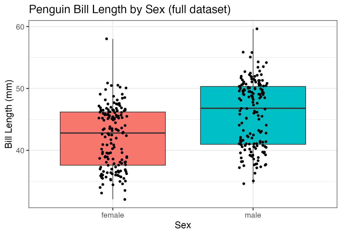
And perform the t-test with the larger sample:
penguins |>
  drop_na() |>
  summarize(t_test = list(t.test(bill_length_mm ~ sex))) |>
  mutate(ttest = map(t_test, tidy)) |>
  unnest(ttest)
You’ll notice that with more data points, our statistical power increases, often leading to more precise estimates and potentially different conclusions about statistical significance.
Summary
T-tests are powerful tools for comparing means between two groups. Key takeaways include:
- Use
t.test()for basic comparisons between two groups - The
broom::tidy()function makes results easier to work with programmatically - Sample size greatly affects your ability to detect differences
- Always visualize your data alongside statistical tests to better understand your results
- Formula notation (
y ~ x) is often more convenient when working with data frames
Remember that statistical significance doesn’t always mean practical significance, so consider the effect size and context of your data when interpreting results.