How to run multiple t-tests using tidyverse in R
Introduction
A t-test is one of the most commonly used statistical tests for determining if there is a significant difference between the means of two groups. This tutorial demonstrates how to perform multiple t-tests efficiently using the tidyverse framework in R, which is particularly useful when you need to compare groups across different categories or subsets of your data.
Loading Required Libraries
First, let’s load the necessary libraries for our analysis:
library(palmerpenguins)
library(tidyverse)
library(broom)
theme_set(theme_bw(16))
We’ll use the palmerpenguins dataset, tidyverse for data manipulation, and broom to convert statistical test outputs into tidy data frames.
Understanding the Data
Let’s start by examining our dataset and creating a sample for initial exploration:
set.seed(42)
df <- penguins |>
  drop_na() |>
  group_by(species) |>
  slice_sample(n = 10) |>
  ungroup()
This code creates a balanced sample of 10 penguins from each species, which helps us understand the analysis workflow before applying it to the full dataset.
df |> head()Visualizing the Data
Before conducting statistical tests, it’s important to visualize our data to understand the distributions and potential differences:
df |>
  ggplot(aes(x = sex, y = bill_length_mm, fill = sex)) +
  geom_boxplot(outlier.shape = NA) +
  geom_jitter(width = 0.1) +
  facet_wrap(~species) +
  theme(legend.position = "none") +
  scale_fill_brewer(palette = "Dark2") +
  labs(title = "Bill Length by Sex Across Penguin Species (sample of 10)",
       x = "Sex", y = "Bill Length (mm)")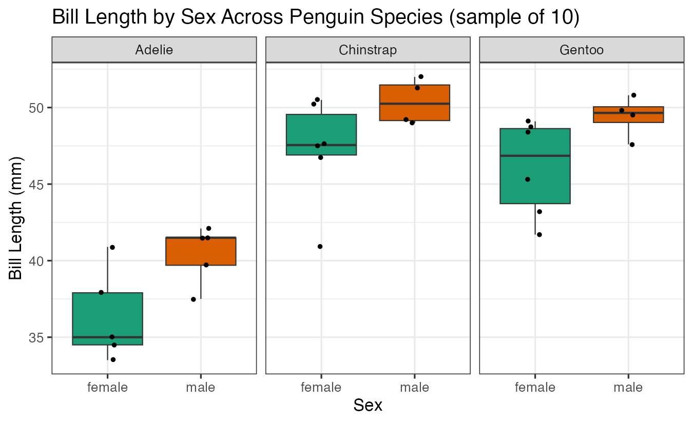
This visualization shows the distribution of bill lengths between male and female penguins for each species, helping us identify potential differences that we can test statistically.
Building the T-Test Workflow Step by Step
The key to performing multiple t-tests with tidyverse is using the list() function to store test objects within grouped data. Let’s build this step by step.
First, let’s group our data by species:
df |>
  group_by(species)
Next, we’ll perform a t-test for each species and store the results as list objects:
df |>
  group_by(species) |>
  summarize(t_test_obj = list(t.test(bill_length_mm ~ sex)))
The list() function allows us to store complex objects (like t-test results) within a data frame. Each row now contains a complete t-test object.
Now we’ll use the broom package to convert these test objects into tidy data frames:
df |>
  group_by(species) |>
  summarize(t_test_obj = list(t.test(bill_length_mm ~ sex))) |>
  mutate(ttest_res = map(t_test_obj, tidy))
The map() function applies the tidy() function to each t-test object, creating a consistent data structure.
Finally, we’ll unnest the results to create a clean, readable output:
df |>
  group_by(species) |>
  summarize(t_test_obj = list(t.test(bill_length_mm ~ sex))) |>
  mutate(ttest_res = map(t_test_obj, tidy)) |>
  unnest(ttest_res)
This final step expands our nested data frames into a single table with one row per species, containing all the t-test statistics including p-values, confidence intervals, and effect estimates.
Applying to the Full Dataset
Now let’s apply our workflow to the complete penguins dataset. First, let’s visualize the full data:
penguins |>
  drop_na() |>
  ggplot(aes(x = sex, y = bill_length_mm, fill = sex)) +
  geom_boxplot(outlier.shape = NA) +
  geom_jitter(width = 0.1) +
  facet_wrap(~species) +
  theme(legend.position = "none") +
  scale_fill_brewer(palette = "Dark2") +
  labs(title = "Bill Length by Sex Across Penguin Species (full dataset)",
       x = "Sex", y = "Bill Length (mm)")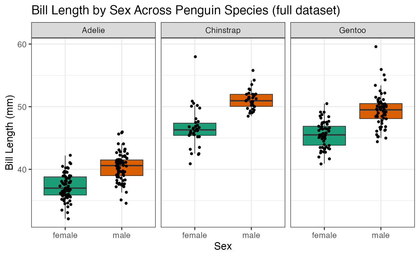
With more data points, we can see clearer patterns in the differences between male and female penguins across species.
Now let’s perform the t-tests on the full dataset:
penguins |>
  drop_na() |>
  group_by(species) |>
  summarize(t_test_obj = list(t.test(bill_length_mm ~ sex))) |>
  mutate(ttest_res = map(t_test_obj, tidy)) |>
  unnest(ttest_res)
The results show statistical comparisons for bill length differences between sexes within each penguin species, including p-values and confidence intervals.
Testing Multiple Variables
We can easily extend this approach to test multiple variables. Let’s examine flipper length:
penguins |>
  drop_na() |>
  ggplot(aes(x = sex, y = flipper_length_mm, fill = sex)) +
  geom_boxplot(outlier.shape = NA) +
  geom_jitter(width = 0.1) +
  facet_wrap(~species) +
  theme(legend.position = "none") +
  scale_fill_brewer(palette = "Dark2") +
  labs(title = "Flipper Length by Sex Across Penguin Species",
       x = "Sex", y = "Flipper Length (mm)")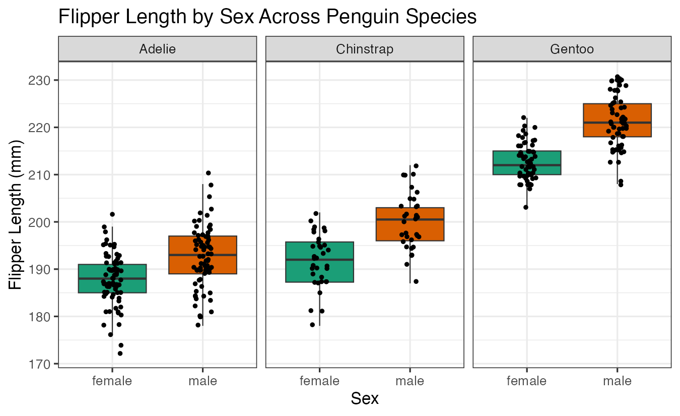
And perform the corresponding t-tests:
penguins |>
  drop_na() |>
  group_by(species) |>
  summarize(t_test = list(t.test(flipper_length_mm ~ sex))) |>
  mutate(ttest = map(t_test, tidy)) |>
  unnest(ttest)
Finally, let’s examine body mass differences:
penguins |>
  drop_na() |>
  ggplot(aes(x = sex, y = body_mass_g, fill = sex)) +
  geom_boxplot(outlier.shape = NA) +
  geom_jitter(width = 0.1) +
  facet_wrap(~species) +
  theme(legend.position = "none") +
  scale_fill_brewer(palette = "Dark2") +
  labs(title = "Body Mass by Sex Across Penguin Species",
       x = "Sex", y = "Body Mass (g)")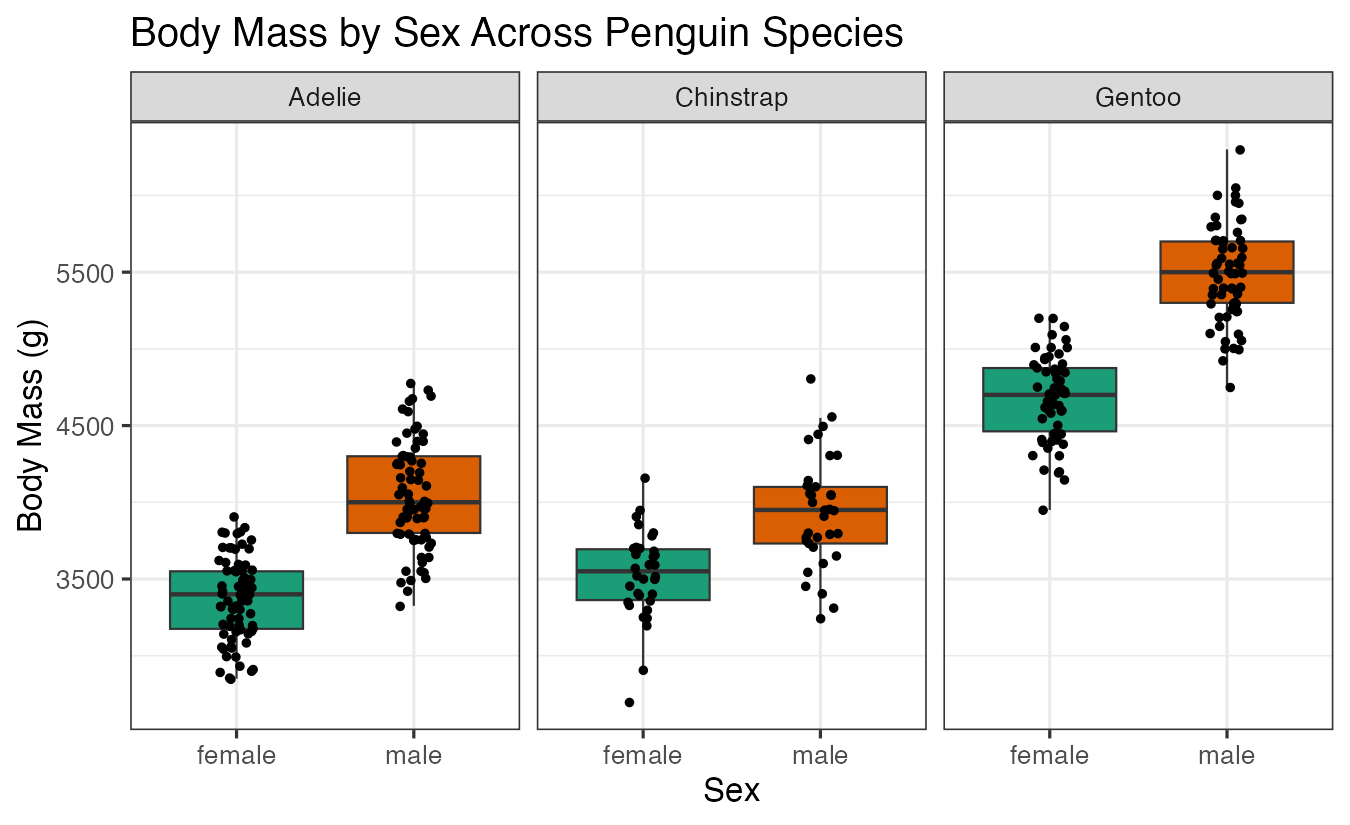
penguins |>
  drop_na() |>
  group_by(species) |>
  summarize(t_test = list(t.test(body_mass_g ~ sex))) |>
  mutate(ttest = map(t_test, tidy)) |>
  unnest(ttest)
These results reveal which morphological features show significant sexual dimorphism within each penguin species.
Summary
This tutorial demonstrated how to efficiently perform multiple t-tests using the tidyverse framework. The key steps involve: (1) grouping data by categories, (2) storing t-test objects in list columns, (3) using map() and tidy() to extract results, and (4) unnesting for clean output. This approach scales well for comparing multiple variables across different groups and provides a reproducible workflow for statistical analysis in R.