library(tidyverse)
library(scales)
theme_set(theme_minimal(base_size = 14))Understanding the Normal Distribution in R
statistics
distributions
ggplot2
Learn about the normal distribution (bell curve) in R with practical examples and visualizations using ggplot2.
What is the Normal Distribution?
The normal distribution, also called the Gaussian distribution or “bell curve,” is one of the most important probability distributions in statistics. It describes how data tends to cluster around a central value (the mean) with symmetric tails on either side.
Many natural phenomena follow a normal distribution: human heights, test scores, measurement errors, and countless other variables. Understanding the normal distribution is fundamental to statistical analysis.
Key Properties
A normal distribution is defined by two parameters:
- Mean (μ): The center of the distribution
- Standard Deviation (σ): How spread out the data is
The famous 68-95-99.7 rule states that: - 68% of data falls within 1 standard deviation of the mean - 95% falls within 2 standard deviations - 99.7% falls within 3 standard deviations
Visualizing the Normal Distribution
Let’s create a visualization of a standard normal distribution (mean=0, sd=1):
x <- seq(-4, 4, length.out = 1000)
y <- dnorm(x, mean = 0, sd = 1)
normal_data <- tibble(x = x, y = y)

# Plot the bell curve
ggplot(normal_data, aes(x = x, y = y)) +
  geom_line(color = "#2563eb", linewidth = 1.2) +
  geom_area(alpha = 0.3, fill = "#2563eb") +
  geom_vline(xintercept = 0, linetype = "dashed", color = "red") +
  labs(
    title = "The Standard Normal Distribution",
    subtitle = "Mean = 0, Standard Deviation = 1",
    x = "Standard Deviations from Mean",
    y = "Probability Density"
  ) +
  scale_x_continuous(breaks = -4:4) +
  annotate("text", x = 0, y = 0.42, label = "μ = 0", color = "red", fontface = "bold")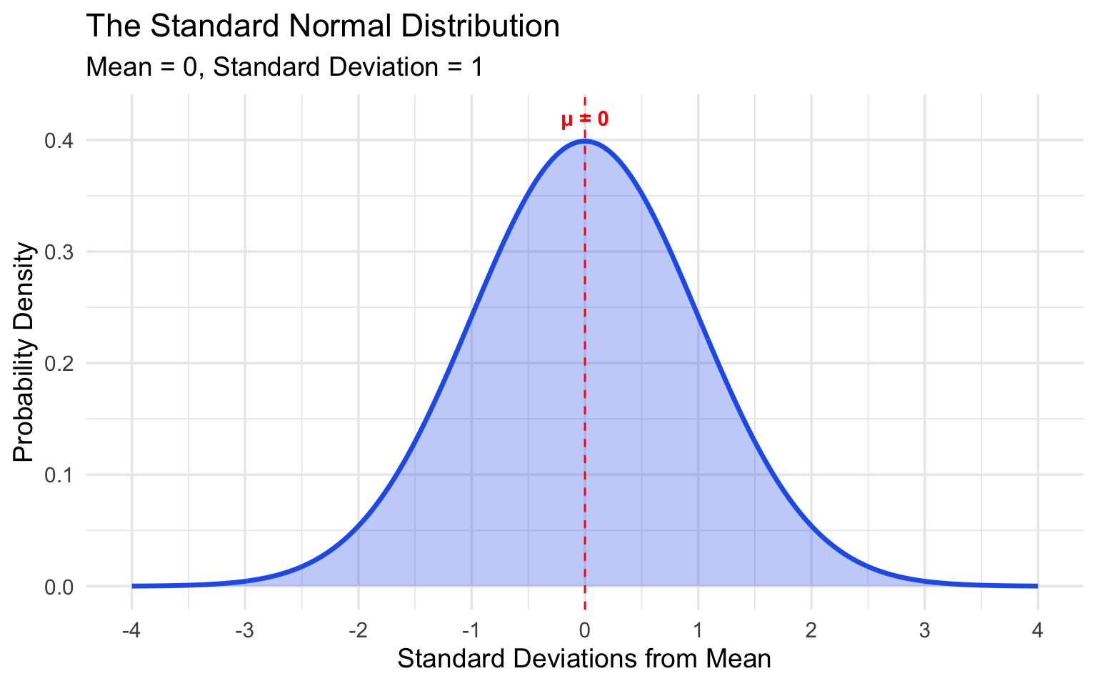
The 68-95-99.7 Rule Visualized
# Create shaded regions for different standard deviations
ggplot(normal_data, aes(x = x, y = y)) +
  # 3 SD region (99.7%)
  geom_area(data = filter(normal_data, x >= -3 & x <= 3),
            fill = "#fef3c7", alpha = 0.8) +
  # 2 SD region (95%)
  geom_area(data = filter(normal_data, x >= -2 & x <= 2),
            fill = "#fde68a", alpha = 0.8) +
  # 1 SD region (68%)
  geom_area(data = filter(normal_data, x >= -1 & x <= 1),
            fill = "#fbbf24", alpha = 0.8) +
  geom_line(color = "#1e3a5f", linewidth = 1.2) +
  geom_vline(xintercept = c(-3, -2, -1, 0, 1, 2, 3),
             linetype = "dashed", alpha = 0.5) +
  labs(
    title = "The 68-95-99.7 Rule",
    subtitle = "Percentage of data within each standard deviation range",
    x = "Standard Deviations from Mean",
    y = "Probability Density"
  ) +
  annotate("text", x = 0, y = 0.15, label = "68%", size = 6, fontface = "bold") +
  annotate("text", x = 1.5, y = 0.05, label = "95%", size = 5) +
  annotate("text", x = 2.5, y = 0.02, label = "99.7%", size = 4) +
  scale_x_continuous(breaks = -4:4)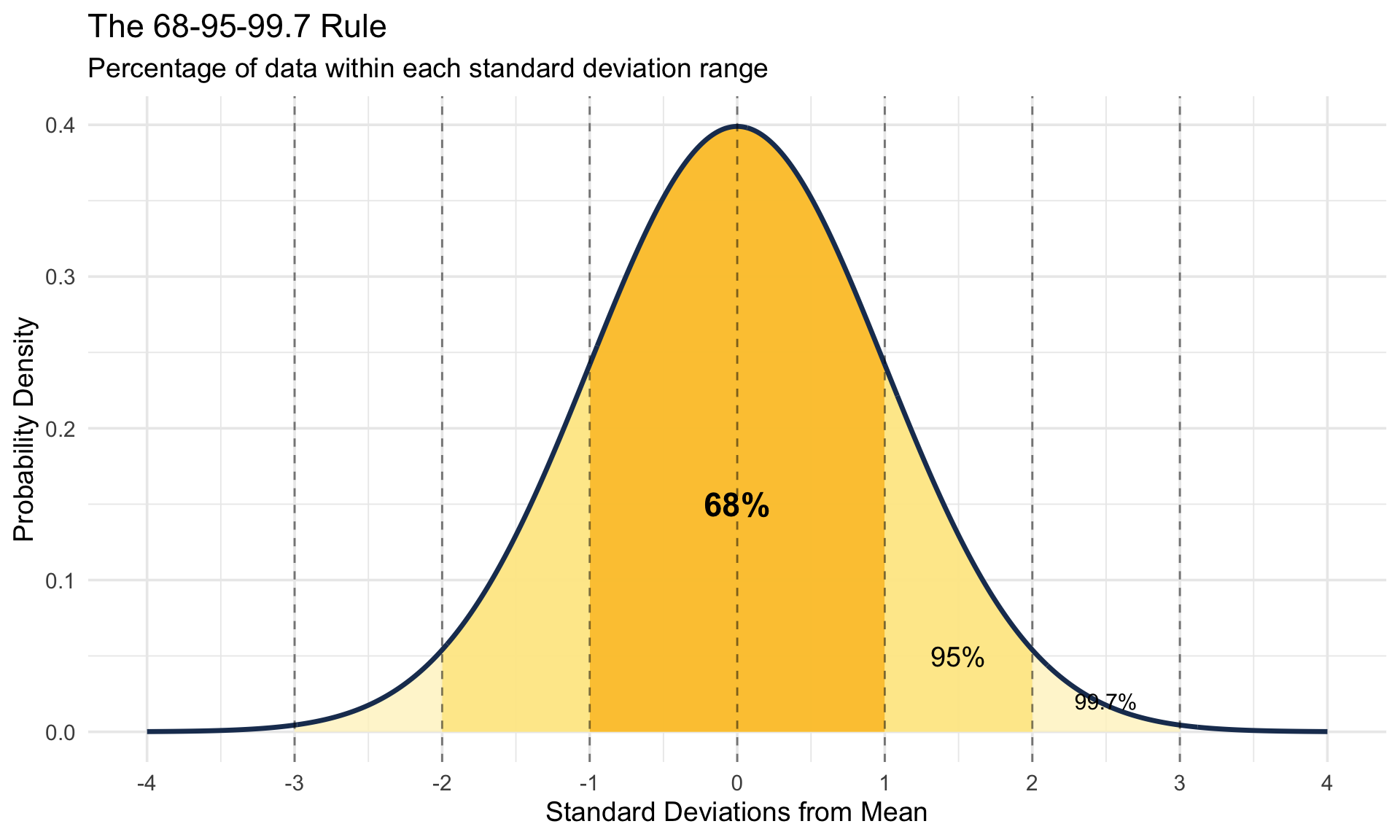
Working with Real Data: Diamond Prices
Let’s explore whether diamond prices follow a normal distribution using the diamonds dataset:
# Examine the diamonds dataset
diamonds |>
  select(carat, cut, price) |>
  head(10)
# A tibble: 10 × 3
carat cut price
<dbl> <ord> <int>
1 0.23 Ideal 326
2 0.21 Premium 326
3 0.23 Good 327
4 0.29 Premium 334
5 0.31 Good 335
6 0.24 Very Good 336
7 0.24 Very Good 336
8 0.26 Very Good 337
9 0.22 Fair 337
10 0.23 Very Good 338diamonds |>
ggplot(aes(x = price)) +
geom_histogram(bins = 50, fill = "#6366f1", color = "white", alpha = 0.8) +
labs(
title = "Distribution of Diamond Prices",
subtitle = "Right-skewed distribution - not normal!",
x = "Price (USD)",
y = "Count"
) +
scale_x_continuous(labels = dollar_format())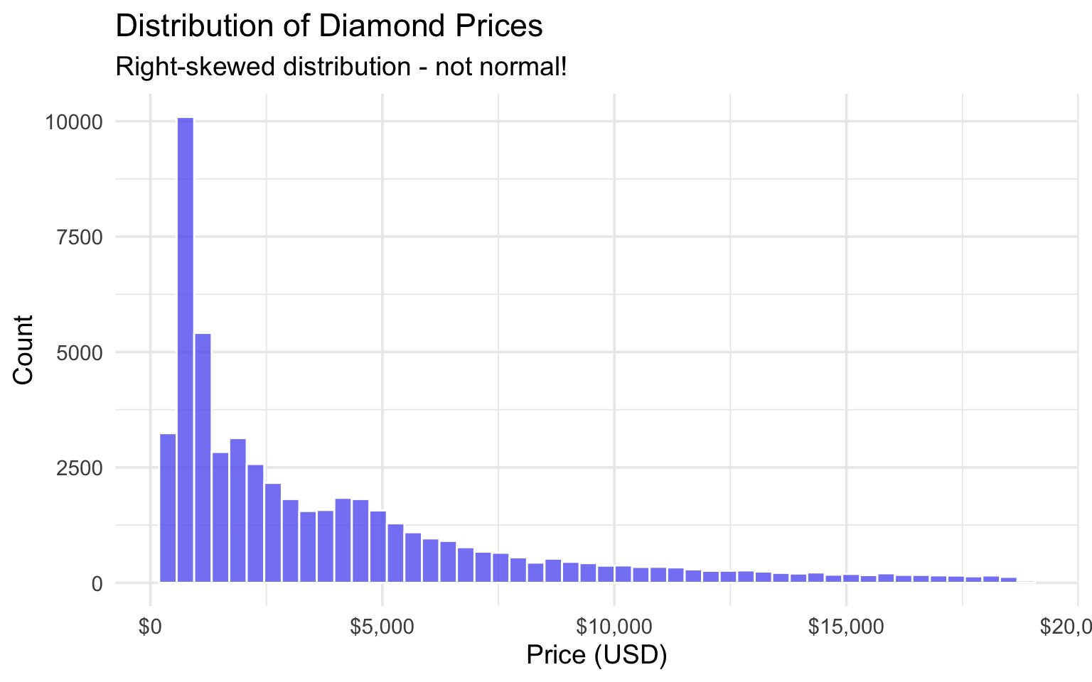
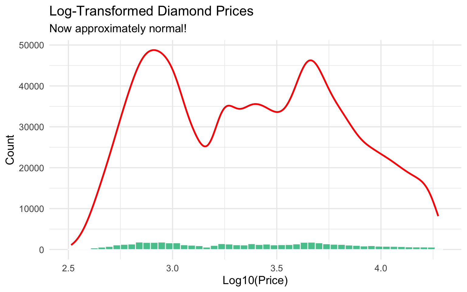
The price distribution is right-skewed, not normal. Let’s try log-transforming it:
diamonds |>
  ggplot(aes(x = log10(price))) +
  geom_histogram(bins = 50, fill = "#10b981", color = "white", alpha = 0.8) +
  geom_density(aes(y = after_stat(count)), color = "red", linewidth = 1) +
  labs(
    title = "Log-Transformed Diamond Prices",
    subtitle = "Now approximately normal!",
    x = "Log10(Price)",
    y = "Count"
  )
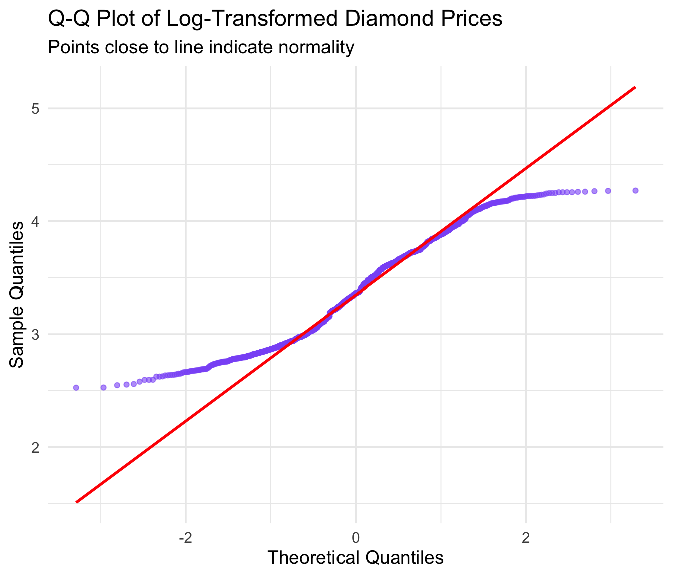
Checking Normality with Q-Q Plots
A Q-Q plot (quantile-quantile plot) is a powerful way to check if data follows a normal distribution. If the points fall along the diagonal line, the data is approximately normal.
diamonds |>
  sample_n(1000) |>  # Sample for faster plotting
  ggplot(aes(sample = log10(price))) +
  stat_qq(color = "#8b5cf6", alpha = 0.6) +
  stat_qq_line(color = "red", linewidth = 1) +
  labs(
    title = "Q-Q Plot of Log-Transformed Diamond Prices",
    subtitle = "Points close to line indicate normality",
    x = "Theoretical Quantiles",
    y = "Sample Quantiles"
  )
Comparing Different Distributions
Let’s compare how different mean and standard deviation values affect the shape:
# Create data for multiple normal distributions
distributions <- tibble(
  x = rep(seq(-10, 15, length.out = 500), 4),
  Distribution = rep(c("μ=0, σ=1", "μ=0, σ=2", "μ=5, σ=1", "μ=2, σ=3"), each = 500)
) |>
  mutate(
    y = case_when(
      Distribution == "μ=0, σ=1" ~ dnorm(x, 0, 1),
      Distribution == "μ=0, σ=2" ~ dnorm(x, 0, 2),
      Distribution == "μ=5, σ=1" ~ dnorm(x, 5, 1),
      Distribution == "μ=2, σ=3" ~ dnorm(x, 2, 3)
    )
  )

ggplot(distributions, aes(x = x, y = y, color = Distribution)) +
  geom_line(linewidth = 1.2) +
  labs(
    title = "Normal Distributions with Different Parameters",
    subtitle = "See how mean shifts the center and SD affects the spread",
    x = "Value",
    y = "Probability Density"
  ) +
  scale_color_brewer(palette = "Set1") +
  theme(legend.position = "top")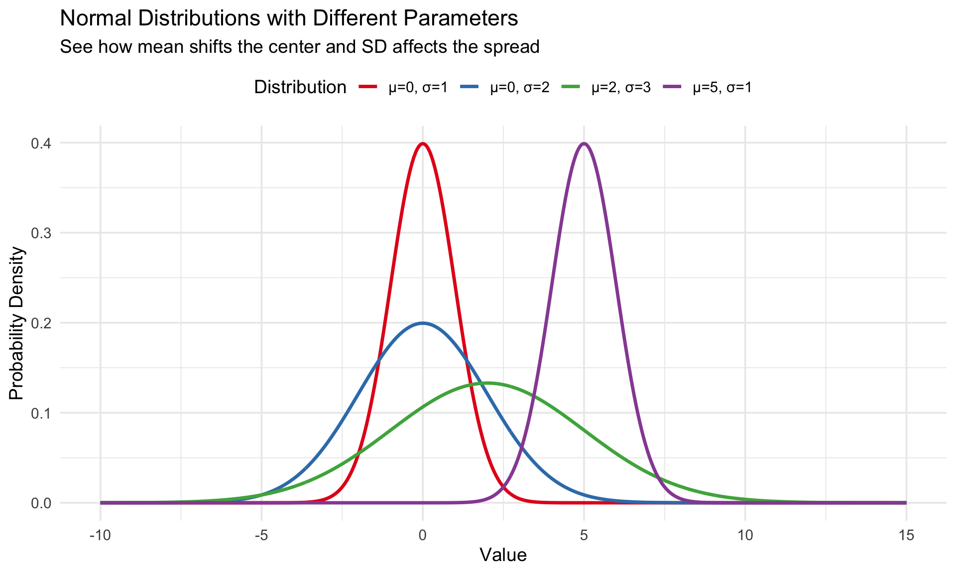
Key R Functions for Normal Distribution
| Function | Description | Example |
|---|---|---|
dnorm() |
Probability density | dnorm(0, mean=0, sd=1) |
pnorm() |
Cumulative probability | pnorm(1.96) → 0.975 |
qnorm() |
Quantile function | qnorm(0.975) → 1.96 |
rnorm() |
Random sampling | rnorm(100, mean=50, sd=10) |
# Probability that Z < 1.96
pnorm(1.96)
[1] 0.9750021# What value gives 95% of data below it?
qnorm(0.95)[1] 1.644854# Generate 10 random values from N(100, 15)
set.seed(42)
rnorm(10, mean = 100, sd = 15) [1] 120.56438 91.52953 105.44693 109.49294 106.06402 98.40813 122.67283
[8] 98.58011 130.27636 99.05929Statistical Test: Shapiro-Wilk
The Shapiro-Wilk test formally tests whether data is normally distributed:
# Test if log-prices are normal (sample required for large datasets)
sample_prices <- diamonds |>
  sample_n(5000) |>
  pull(price)

# Original prices - not normal
shapiro.test(sample_prices)
    Shapiro-Wilk normality test

data:  sample_prices
W = 0.79619, p-value < 2.2e-16
# Log-transformed - closer to normal
shapiro.test(log10(sample_prices))
    Shapiro-Wilk normality test

data:  log10(sample_prices)
W = 0.9663, p-value < 2.2e-16
A small p-value (< 0.05) suggests the data is not normally distributed.
Summary
- The normal distribution is defined by mean and standard deviation
- Use
dnorm(),pnorm(),qnorm(),rnorm()for calculations - Check normality with histograms, Q-Q plots, and Shapiro-Wilk test
- Many statistical tests assume normality - always check your data!
- Log transformation can help normalize right-skewed data