How to perform t-test in R
Introduction
A t-test is a statistical test used to compare means between groups or against a known value. It’s essential for determining whether observed differences are statistically significant or due to random chance.
Getting Started
library(tidyverse)
library(palmerpenguins)
Example 1: Basic Usage
The Problem
We want to test if the average body mass of Adelie penguins differs significantly from 4000 grams. This is a one-sample t-test comparing our sample mean to a known value.
Step 1: Prepare the data
First, we’ll filter our dataset to focus on Adelie penguins only.
adelie_data <- penguins |>
  filter(species == "Adelie") |>
  drop_na(body_mass_g)

head(adelie_data)
This creates a clean dataset with 146 Adelie penguins, removing any missing body mass values.
Step 2: Explore the data
Let’s examine the distribution and calculate basic statistics.
adelie_data |>
  summarise(
    mean_mass = mean(body_mass_g),
    sd_mass = sd(body_mass_g),
    n = n()
  )
The average body mass is approximately 3706 grams, which appears different from our test value of 4000 grams.
Step 3: Perform one-sample t-test
Now we’ll conduct the statistical test to determine if this difference is significant.
t_result <- t.test(adelie_data$body_mass_g,
                   mu = 4000)
print(t_result)
The p-value is much less than 0.05, indicating that Adelie penguins have significantly different body mass from 4000 grams.
Example 2: Practical Application
The Problem
A researcher wants to compare flipper lengths between male and female Adelie penguins. This requires a two-sample t-test to determine if there’s a significant difference between the two groups.
Step 1: Prepare comparison data
We’ll filter for Adelie penguins and remove any missing values for sex and flipper length.
adelie_comparison <- penguins |>
  filter(species == "Adelie") |>
  drop_na(sex, flipper_length_mm)

head(adelie_comparison)
This gives us a clean dataset ready for comparing flipper lengths between sexes.
Step 2: Visualize the differences
Before testing, let’s visualize the data to understand the distributions.
adelie_comparison |>
  ggplot(aes(x = sex, y = flipper_length_mm, fill = sex)) +
  geom_boxplot(alpha = 0.7, outlier.shape = NA) +
  geom_jitter(width = 0.15, alpha = 0.6) +
  labs(title = "Flipper Length by Sex in Adelie Penguins",
       subtitle = "Two-sample t-test of flipper length by sex",
       x = "Sex", y = "Flipper Length (mm)") +
  theme_minimal() +
  theme(legend.position = "none")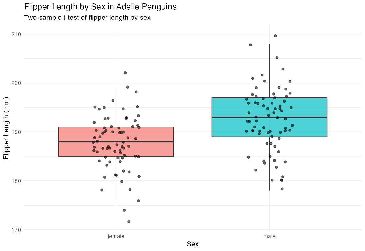
The boxplot suggests male penguins have longer flippers than females, but we need statistical confirmation.
Step 3: Calculate group statistics
Let’s examine the summary statistics for each group.
adelie_comparison |>
  group_by(sex) |>
  summarise(
    mean_flipper = mean(flipper_length_mm),
    sd_flipper = sd(flipper_length_mm),
    n = n()
  )
Males show higher average flipper length (approximately 192mm) compared to females (approximately 188mm).
Step 4: Perform two-sample t-test
Now we’ll test if this observed difference is statistically significant.
t_test_two_sample <- t.test(flipper_length_mm ~ sex,
                           data = adelie_comparison)
print(t_test_two_sample)
The p-value indicates whether the difference in flipper lengths between sexes is statistically significant.
Step 5: Interpret results
Let’s extract key information from our test results.
# Extract confidence interval and p-value
cat("P-value:", t_test_two_sample$p.value, "\n")
cat("95% Confidence Interval:",
    t_test_two_sample$conf.int[1], "to",
    t_test_two_sample$conf.int[2])
These results help us make informed conclusions about the difference between male and female flipper lengths.
Summary
- One-sample t-tests compare a sample mean against a known value using
t.test(data, mu = value) - Two-sample t-tests compare means between two groups using
t.test(variable ~ group, data = dataset) - P-values less than 0.05 typically indicate statistically significant differences
- Always explore your data visually before conducting statistical tests
The
t.test()function provides confidence intervals, test statistics, and p-values for interpretation