How to use geom_area() in R
Introduction
The geom_area() function in ggplot2 creates area plots by filling the area between a line and the x-axis. It’s particularly useful for visualizing cumulative data, showing proportions over time, or creating stacked area charts. Area plots help emphasize the magnitude of values and make it easy to see trends in continuous data.
Getting Started
library(tidyverse)
library(palmerpenguins)
Example 1: Basic Area Plot
The Problem
We want to create a simple area plot showing the cumulative distribution of penguin body masses. This will help us visualize how the data accumulates across different weight ranges.
Step 1: Prepare the data
First, we’ll create a density distribution of penguin body masses.
penguin_density <- penguins |>
  filter(!is.na(body_mass_g)) |>
  pull(body_mass_g) |>
  density()
This creates a density object that we can convert into a data frame for plotting.
Step 2: Convert to data frame
We need to transform the density data into a format ggplot2 can work with.
density_df <- data.frame(
  x = penguin_density$x,
  y = penguin_density$y
)
Now we have x and y coordinates representing the density curve of body masses.
Step 3: Create the basic area plot
Let’s create our first area plot using the density data.
ggplot(density_df, aes(x = x, y = y)) +
  geom_area(fill = "skyblue", alpha = 0.7) +
  labs(title = "Distribution of Penguin Body Mass",
       x = "Body Mass (g)", y = "Density")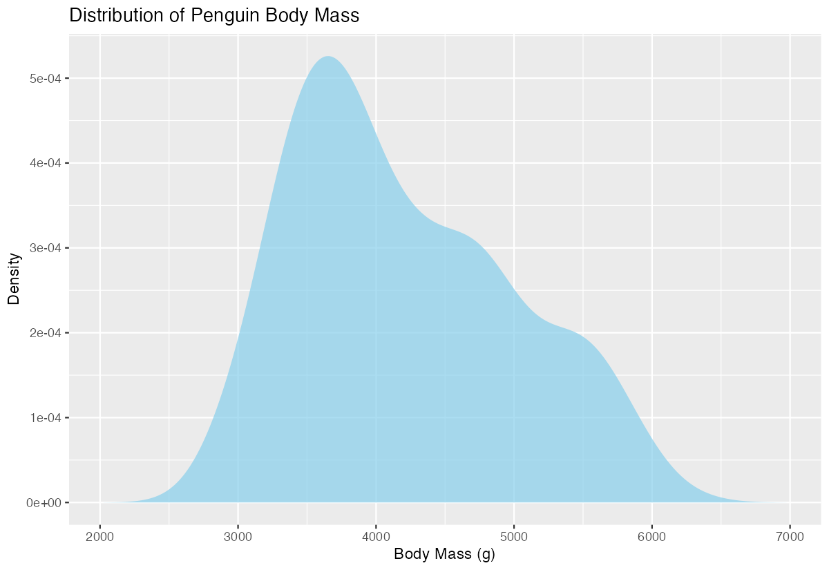
The area under the curve is now filled, making it easy to see the overall distribution shape.
Example 2: Stacked Area Chart with Multiple Groups
The Problem
We want to compare how penguin body mass distributions vary by species over time. A stacked area chart will show both individual species contributions and the total combined distribution, which is perfect for understanding composition and trends.
Step 1: Create sample time series data
We’ll simulate monthly data showing penguin populations by species.
time_data <- expand.grid(
  month = 1:12,
  species = c("Adelie", "Chinstrap", "Gentoo")
) |>
  mutate(population = case_when(
    species == "Adelie" ~ 100 + month * 5 + rnorm(36, 0, 10),
    species == "Chinstrap" ~ 60 + month * 3 + rnorm(36, 0, 8),
    species == "Gentoo" ~ 80 + month * 4 + rnorm(36, 0, 12)
  ))
This creates realistic population data that varies by month and species.
Step 2: Create the stacked area plot
Now we’ll build a stacked area chart to show population changes over time.
ggplot(time_data, aes(x = month, y = population, fill = species)) +
  geom_area(position = "stack", alpha = 0.8) +
  scale_fill_manual(values = c("Adelie" = "#FF6B6B",
                               "Chinstrap" = "#4ECDC4",
                               "Gentoo" = "#45B7D1"))
The stacked areas show both individual species trends and total population growth.
Step 3: Enhance with better formatting
Let’s improve the plot with better labels and theme.
time_data |>
  ggplot(aes(x = month, y = population, fill = species)) +
  geom_area(position = "stack", alpha = 0.8) +
  scale_fill_manual(values = c("Adelie" = "#FF6B6B",
                               "Chinstrap" = "#4ECDC4",
                               "Gentoo" = "#45B7D1")) +
  labs(title = "Penguin Population by Species Over Time",
       x = "Month", y = "Population", fill = "Species") +
  theme_minimal()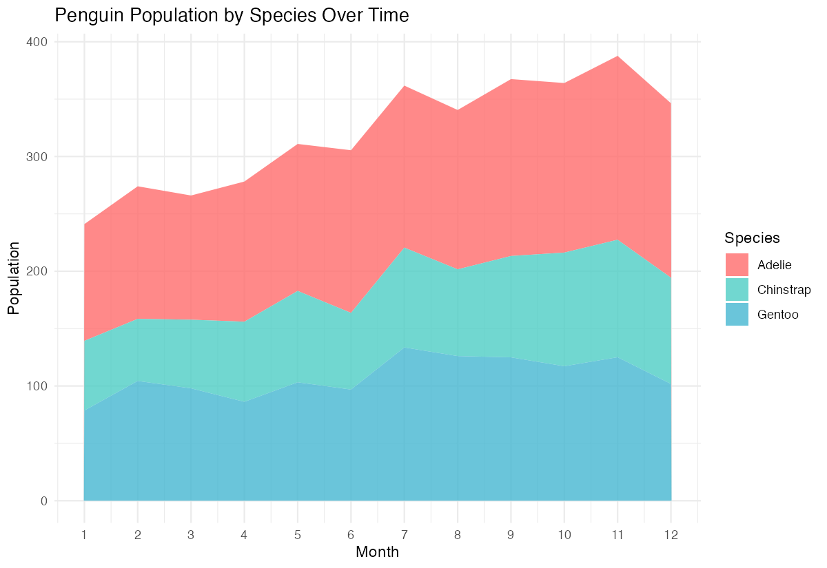
The final plot clearly shows how each species contributes to the total population throughout the year.
Step 4: Create proportional area chart
For better comparison, we can show relative proportions instead of absolute numbers.
time_data |>
  ggplot(aes(x = month, y = population, fill = species)) +
  geom_area(position = "fill", alpha = 0.8) +
  scale_fill_manual(values = c("Adelie" = "#FF6B6B",
                               "Chinstrap" = "#4ECDC4",
                               "Gentoo" = "#45B7D1")) +
  labs(title = "Relative Penguin Population Proportions",
       x = "Month", y = "Proportion", fill = "Species")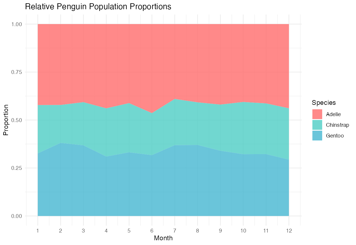
Using position = "fill" shows each species as a proportion of the total, making relative changes more apparent.
Summary
- Basic area plots use
geom_area()to fill the area under a curve, perfect for showing distributions or cumulative data - Stacked area charts with
position = "stack"display multiple groups while showing both individual and total values - Proportional area charts with
position = "fill"emphasize relative contributions rather than absolute values - Customize appearance using
fill,alpha, andscale_fill_manual()to create visually appealing and informative plots Area plots work best with continuous x-axis data and are particularly effective for time series or cumulative datasets