How to use geom_tile() in R
Introduction
The geom_tile() function in ggplot2 creates rectangular tiles or heatmaps by plotting filled rectangles at specified x and y coordinates. This visualization is particularly useful for displaying correlations, creating calendar heatmaps, or showing relationships between categorical variables through color intensity.
Getting Started
library(tidyverse)
library(palmerpenguins)
Example 1: Basic Usage
The Problem
We want to create a simple heatmap showing the relationship between two categorical variables. Let’s visualize how penguin species are distributed across different islands using tile colors.
Step 1: Prepare the data
We need to count the number of penguins by species and island to create our tile data.
penguin_counts <- penguins |>
  filter(!is.na(species), !is.na(island)) |>
  count(species, island, name = "count")

penguin_counts
This creates a summary table with species, island, and the count of penguins for each combination.
Step 2: Create basic tiles
Now we’ll create our first heatmap using geom_tile() with the count values determining the fill color.
ggplot(penguin_counts, aes(x = island, y = species)) +
  geom_tile(aes(fill = count)) +
  labs(title = "Penguin Distribution by Species and Island")
The tiles show darker colors for higher penguin counts, creating an immediate visual representation of the distribution patterns.
Step 3: Improve the appearance
Let’s enhance the visualization with better colors and formatting.
ggplot(penguin_counts, aes(x = island, y = species)) +
  geom_tile(aes(fill = count), color = "white", linewidth = 0.5) +
  scale_fill_gradient(low = "lightblue", high = "darkblue") +
  labs(title = "Penguin Distribution by Species and Island",
       x = "Island", y = "Species", fill = "Count") +
  theme_minimal()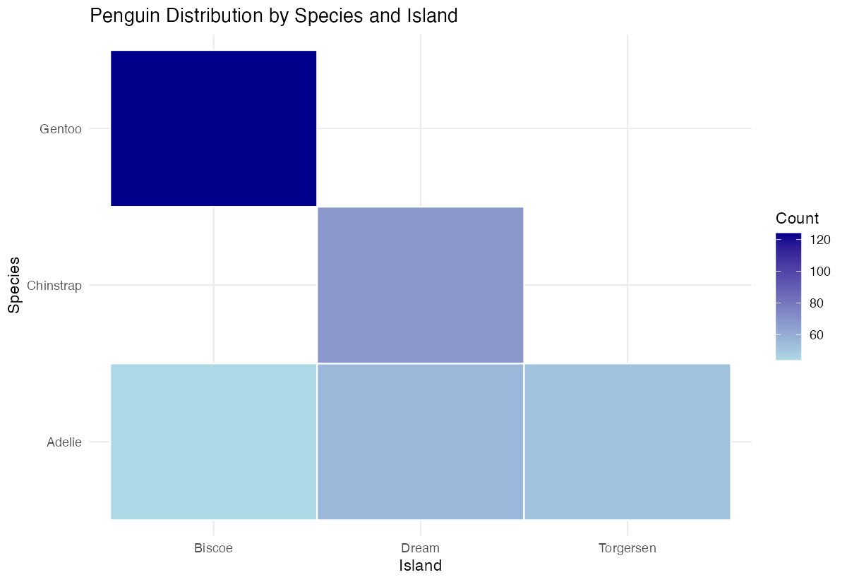
The white borders and improved color scheme make the tiles more distinct and visually appealing.
Example 2: Practical Application
The Problem
We want to create a correlation heatmap to understand relationships between numeric variables in our dataset. This is commonly used in data analysis to identify which variables are strongly related to each other.
Step 1: Calculate correlations
First, we’ll compute correlations between numeric penguin measurements.
penguin_cor <- penguins |>
  select(bill_length_mm, bill_depth_mm,
         flipper_length_mm, body_mass_g) |>
  na.omit() |>
  cor()
This creates a correlation matrix showing how each numeric variable relates to the others.
Step 2: Convert to long format
We need to reshape the correlation matrix for use with ggplot2.
cor_data <- penguin_cor |>
  as.data.frame() |>
  rownames_to_column("var1") |>
  pivot_longer(-var1, names_to = "var2", values_to = "correlation")
The long format allows ggplot2 to properly map variables to x and y aesthetics.
Step 3: Create correlation heatmap
Now we’ll build a professional-looking correlation heatmap.
ggplot(cor_data, aes(x = var1, y = var2)) +
  geom_tile(aes(fill = correlation)) +
  scale_fill_gradient2(low = "red", mid = "white", high = "blue",
                       midpoint = 0) +
  theme_minimal()
The diverging color scale helps identify positive (blue) and negative (red) correlations clearly.
Step 4: Add correlation values
Let’s include the actual correlation values on each tile for precise reading.
ggplot(cor_data, aes(x = var1, y = var2)) +
  geom_tile(aes(fill = correlation)) +
  geom_text(aes(label = round(correlation, 2)), color = "black") +
  scale_fill_gradient2(low = "red", mid = "white", high = "blue",
                       midpoint = 0)
The text labels provide exact correlation values while maintaining the visual impact of the color coding.
Step 5: Polish the final visualization
Finally, let’s improve the labels and overall appearance.
ggplot(cor_data, aes(x = var1, y = var2)) +
  geom_tile(aes(fill = correlation), color = "gray") +
  geom_text(aes(label = round(correlation, 2))) +
  scale_fill_gradient2(low = "red", mid = "white", high = "blue", midpoint = 0) +
  labs(title = "Penguin Measurements Correlation Heatmap",
       x = "", y = "", fill = "Correlation") +
  theme_minimal() +
  theme(axis.text.x = element_text(angle = 45, hjust = 1))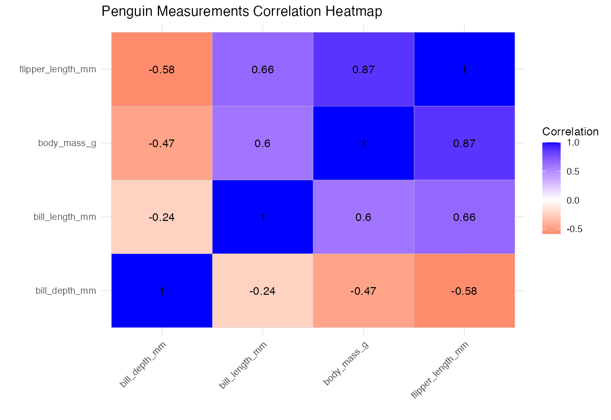
The rotated x-axis labels prevent overlapping and the clean theme creates a professional appearance.
Summary
geom_tile()creates rectangular heatmaps perfect for displaying relationships between categorical or continuous variables- Always prepare your data in the correct format with x, y, and fill variables clearly defined
- Use
scale_fill_gradient()for single-direction color schemes andscale_fill_gradient2()for diverging scales - Add
geom_text()to display exact values on tiles when precision is important White or gray borders between tiles improve readability and visual separation