How to calculate cumulative sum in R
Introduction
Cumulative sum calculates the running total of values in a sequence, where each element represents the sum of all previous elements up to that point. This technique is essential for analyzing trends over time, calculating running totals in financial data, or tracking progressive changes in datasets.
Getting Started
library(tidyverse)
library(palmerpenguins)
Example 1: Basic Usage
The Problem
We need to understand how cumulative sum works with a simple numeric vector. Let’s start with basic numbers to see the cumulative addition process.
Step 1: Create a simple vector
We’ll create a basic numeric vector to demonstrate the concept.
numbers <- c(1, 3, 5, 2, 4)
numbers
This gives us our starting values: 1, 3, 5, 2, 4.
Step 2: Calculate cumulative sum
The cumsum() function calculates the running total at each position.
cumulative_result <- cumsum(numbers)
cumulative_result
The result shows: 1, 4, 9, 11, 15 (1, then 1+3=4, then 4+5=9, etc.).
Step 3: Visualize the difference
Let’s compare original values with their cumulative sums in a data frame.
comparison <- data.frame(
  position = 1:5,
  original = numbers,
  cumulative = cumulative_result
)
comparison
This clearly shows how each cumulative value builds upon the previous total.
Example 2: Practical Application
The Problem
We want to analyze penguin body mass data from Palmer Station, calculating running totals by species. This helps us understand how body mass accumulates when penguins are ordered by measurement date or size.
Step 1: Prepare the penguin data
We’ll filter out missing values and select relevant columns for our analysis.
penguin_data <- penguins |>
  filter(!is.na(body_mass_g)) |>
  select(species, body_mass_g, year) |>
  arrange(species, body_mass_g)
This creates a clean dataset with species, body mass, and year information.
Step 2: Calculate cumulative sum by species
We’ll group by species and calculate cumulative body mass within each group.
penguin_cumsum <- penguin_data |>
  group_by(species) |>
  mutate(
    cumulative_mass = cumsum(body_mass_g),
    penguin_count = row_number()
  )
Now each row shows the running total of body mass for that species.
Step 3: View the results
Let’s examine the first few rows for each species to see the pattern.
penguin_cumsum |>
  group_by(species) |>
  slice_head(n = 5) |>
  select(species, body_mass_g, cumulative_mass, penguin_count)
This shows how cumulative mass increases as we add each penguin’s weight.
Step 4: Create a visualization
We’ll plot the cumulative mass progression for better understanding.
penguin_cumsum |>
  ggplot(aes(x = penguin_count, y = cumulative_mass, color = species)) +
  geom_line() +
  labs(title = "Cumulative Body Mass by Species",
       x = "Number of Penguins", y = "Cumulative Mass (g)")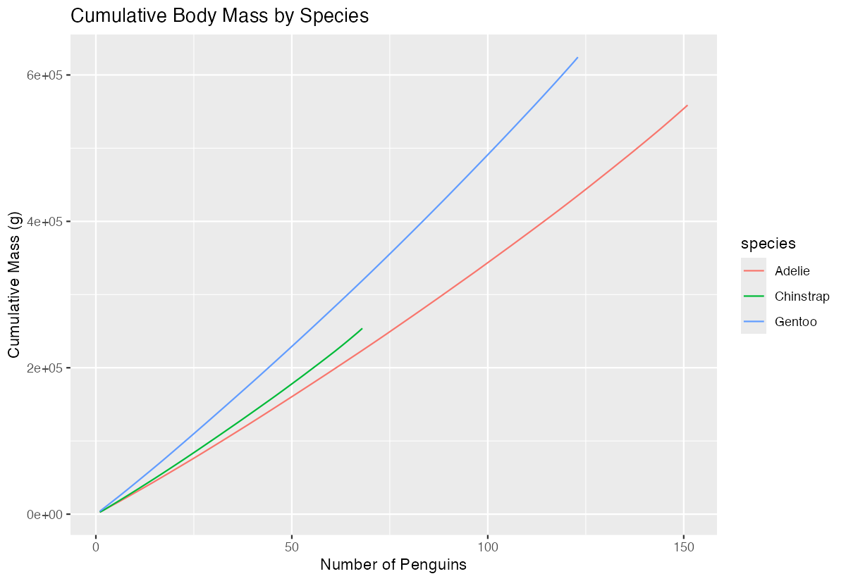
The visualization reveals how quickly total mass accumulates for each species.
Step 5: Calculate cumulative percentage
We can also show what percentage each penguin contributes to the total.
penguin_final <- penguin_cumsum |>
  group_by(species) |>
  mutate(
    total_mass = sum(body_mass_g),
    cumulative_percent = (cumulative_mass / total_mass) * 100
  ) |>
  select(species, body_mass_g, cumulative_percent)
This shows each penguin’s contribution to their species’ total body mass.
Summary
- Use
cumsum()for basic cumulative sum calculations on numeric vectors - Combine
group_by()andmutate()withcumsum()for grouped calculations in data frames - Cumulative sums are perfect for tracking running totals, financial data, and progressive measurements
- The
|>pipe operator makes cumulative sum operations more readable in complex data workflows Visualization helps reveal patterns in cumulative data that aren’t obvious in raw numbers