Computing Correlation Between Multiple Variables in a dataframe
Introduction
Correlation analysis helps you understand relationships between numeric variables in your dataset. Computing correlations across multiple variables simultaneously allows you to quickly identify which variables move together and spot potential patterns in your data.
Getting Started
library(tidyverse)
library(palmerpenguins)
Example 1: Basic Correlation Matrix
The Problem
You have a dataset with several numeric variables and want to see how they correlate with each other. Let’s start with the classic mtcars dataset to compute correlations between all numeric variables.
Step 1: Load and examine the data
First, let’s look at our dataset structure.
data(mtcars)
head(mtcars, 3)
str(mtcars)
We can see mtcars contains 11 numeric variables that we can analyze for correlations.
Step 2: Compute basic correlation matrix
The cor() function calculates correlations between all numeric columns.
correlation_matrix <- mtcars |>
  cor()

correlation_matrix
This produces an 11x11 matrix showing Pearson correlations between every pair of variables, ranging from -1 to 1.
Step 3: Handle missing values
When your data contains NA values, specify how to handle them.
# Remove rows with any missing values
correlation_clean <- mtcars |>
  cor(use = "complete.obs")

# Or use pairwise deletion
correlation_pairwise <- mtcars |>
  cor(use = "pairwise.complete.obs")
The use parameter ensures correlations are calculated properly even with missing data.
Example 2: Practical Application with Real Data
The Problem
You’re analyzing penguin body measurements from the Palmer Penguins dataset. You want to understand which physical characteristics are most strongly related and focus only on the measurement variables.
Step 1: Select and prepare relevant variables
Let’s focus on the four key measurement variables.
penguin_measurements <- penguins |>
  select(bill_length_mm, bill_depth_mm,
         flipper_length_mm, body_mass_g) |>
  drop_na()

glimpse(penguin_measurements)
We now have a clean dataset with four numeric measurement variables and no missing values.
Step 2: Compute correlation matrix with rounded values
Calculate correlations and round for easier interpretation.
penguin_correlations <- penguin_measurements |>
  cor() |>
  round(2)

penguin_correlations
The rounded correlations are much easier to read and interpret than the full decimal values.
Step 3: Convert to tidy format for analysis
Transform the correlation matrix into a long format for further analysis.
penguin_cor_tidy <- penguin_correlations |>
  as.data.frame() |>
  rownames_to_column("var1") |>
  pivot_longer(-var1, names_to = "var2", values_to = "correlation")

head(penguin_cor_tidy)
This tidy format makes it easy to filter, sort, or visualize the correlations.
Step 4: Find strongest correlations
Identify the most interesting relationships by filtering strong correlations.
strong_correlations <- penguin_cor_tidy |>
  filter(var1 != var2) |>  # Remove self-correlations
  filter(abs(correlation) > 0.5) |>
  arrange(desc(abs(correlation)))

strong_correlations
This reveals which penguin measurements are most strongly related to each other.
Step 5: Create a simple correlation heatmap
Visualize the correlation patterns for better understanding.
penguin_cor_tidy |>
  ggplot(aes(var1, var2, fill = correlation)) +
  geom_tile() +
  scale_fill_gradient2(low = "blue", high = "red", mid = "white") +
  theme(axis.text.x = element_text(angle = 45, hjust = 1))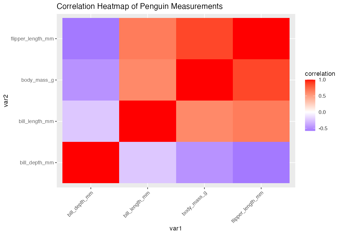
The heatmap provides an intuitive visual representation of which variables correlate positively (red) or negatively (blue).
Summary
- Use
cor()to compute correlation matrices between all numeric variables in a dataframe - Handle missing values with
use = "complete.obs"oruse = "pairwise.complete.obs" - Round correlation values with
round()for easier interpretation - Convert correlation matrices to tidy format using
pivot_longer()for advanced analysis Filter and sort correlations to identify the strongest relationships in your data