Simple linear regression with tidyverse
Introduction
Simple linear regression models the relationship between two continuous variables by fitting a straight line through data points. This technique helps predict one variable based on another and is fundamental for understanding correlations in your data.
Getting Started
library(tidyverse)
library(palmerpenguins)
Example 1: Basic Usage
The Problem
We want to understand if there’s a linear relationship between penguin flipper length and body mass. This will help us predict body mass based on flipper measurements.
Step 1: Explore the Data
First, let’s examine our dataset and visualize the relationship.
penguins |>
  select(flipper_length_mm, body_mass_g) |>
  head(10)
This shows us the structure of our two key variables.
Step 2: Create a Scatter Plot
Visualizing data helps identify linear patterns before modeling.
penguins |>
  ggplot(aes(x = flipper_length_mm, y = body_mass_g)) +
  geom_point() +
  labs(title = "Penguin Flipper Length vs Body Mass")
The scatter plot reveals a clear positive linear relationship between flipper length and body mass.
Step 3: Fit the Linear Model
Now we’ll create our regression model using the lm() function.
model <- penguins |>
  lm(body_mass_g ~ flipper_length_mm, data = _)

summary(model)
The model summary shows coefficients, R-squared value, and statistical significance of our relationship.
Step 4: Add Regression Line to Plot
Visual confirmation helps validate our model’s fit to the data.
penguins |>
  ggplot(aes(x = flipper_length_mm, y = body_mass_g)) +
  geom_point() +
  geom_smooth(method = "lm", se = TRUE) +
  labs(title = "Linear Regression: Flipper Length vs Body Mass")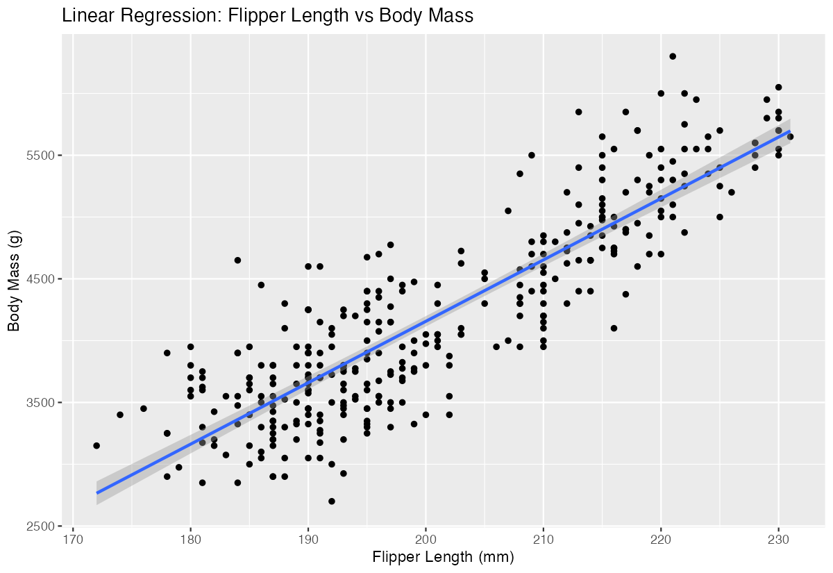
The regression line with confidence bands shows our model fits the data well.
Example 2: Practical Application
The Problem
A marine biologist needs to estimate penguin body mass when only flipper measurements are available in field studies. We’ll build a predictive model and evaluate its accuracy using the mtcars dataset for comparison.
Step 1: Prepare Training Data
We’ll use complete cases and create a clean dataset for modeling.
clean_penguins <- penguins |>
  filter(!is_na(flipper_length_mm), !is_na(body_mass_g)) |>
  select(flipper_length_mm, body_mass_g)

nrow(clean_penguins)
This ensures we have complete data for accurate model training.
Step 2: Build and Extract Model Coefficients
Creating a model with easily interpretable coefficients for field predictions.
field_model <- lm(body_mass_g ~ flipper_length_mm, data = clean_penguins)

coefficients <- field_model |>
  broom::tidy()

coefficients
The coefficients table provides the intercept and slope needed for manual calculations in the field.
Step 3: Make Predictions on New Data
Testing our model’s predictive capability with hypothetical flipper measurements.
new_measurements <- tibble(flipper_length_mm = c(190, 200, 210, 220))

predictions <- new_measurements |>
  mutate(predicted_mass = predict(field_model, newdata = new_measurements))

predictions
These predictions show how body mass increases with flipper length, giving field researchers estimation guidelines.
Step 4: Evaluate Model Performance
Assessing model quality using standard regression diagnostics.
model_stats <- field_model |>
  broom::glance()

model_stats |>
  select(r.squared, adj.r.squared, p.value)
High R-squared values and low p-values indicate our model explains the relationship well and is statistically significant.
Summary
- Simple linear regression with tidyverse uses
lm()combined with pipe operators for clean, readable code - Always visualize your data first with scatter plots to identify linear relationships before modeling
- Use
geom_smooth(method = "lm")to add regression lines to ggplot visualizations - Extract model information using
broom::tidy()andbroom::glance()for tidy data frames Make predictions on new data using
predict()with your fitted model object