Linear regression is a fundamental statistical method that models the relationship between a continuous outcome variable (dependent variable) and one or more…
Published
February 21, 2026
1. Introduction
Linear regression is a fundamental statistical method that models the relationship between a continuous outcome variable (dependent variable) and one or more predictor variables (independent variables). It assumes this relationship can be represented by a straight line, making it one of the most interpretable machine learning techniques.
You would use linear regression when you want to: - Predict a continuous outcome based on other variables - Understand how much each predictor influences the outcome - Test hypotheses about relationships between variables - Create a baseline model for comparison with more complex methods
Linear regression requires several key assumptions: - Linearity: The relationship between predictors and outcome is linear - Independence: Observations are independent of each other - Homoscedasticity: Residuals have constant variance across all fitted values - Normality: Residuals are normally distributed - No multicollinearity: Predictor variables aren’t highly correlated with each other
When these assumptions are met, linear regression provides reliable, interpretable results that form the foundation for more advanced statistical modeling techniques.
2. The Math
The basic linear regression equation is:
Y = β₀ + β₁X₁ + β₂X₂ + ... + βₚXₚ + ε
Where: - Y = the outcome variable we’re trying to predict - β₀ = the intercept (value of Y when all X variables equal zero) - β₁, β₂, βₚ = coefficients showing how much Y changes for a one-unit increase in each X - X₁, X₂, Xₚ = predictor variables - ε = error term (residuals - the difference between predicted and actual values)
For simple linear regression (one predictor), this simplifies to:
Y = β₀ + β₁X + ε
The goal is to find the best-fitting line by minimizing the sum of squared residuals (ordinary least squares). R calculates these coefficients automatically, but understanding what they represent is crucial for interpretation.
3. R Implementation
# Load required packageslibrary(tidyverse)library(palmerpenguins)library(broom)# Load the datadata(penguins)glimpse(penguins)
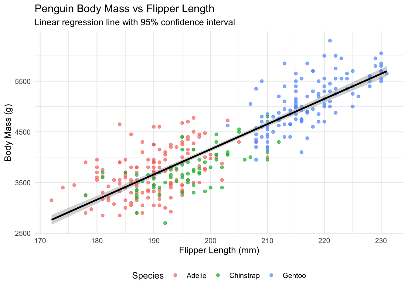
# Load packages for visualizationlibrary(tidyverse)library(palmerpenguins)# Prepare clean datapenguins_clean <- penguins |>filter(!is.na(body_mass_g), !is.na(flipper_length_mm))# Scatter plot with regression lineggplot(penguins_clean, aes(x = flipper_length_mm, y = body_mass_g)) +geom_point(aes(color = species), alpha =0.7) +geom_smooth(method ="lm", se =TRUE, color ="black") +labs(title ="Penguin Body Mass vs Flipper Length",subtitle ="Linear regression line with 95% confidence interval",x ="Flipper Length (mm)",y ="Body Mass (g)",color ="Species" ) +theme_minimal() +theme(legend.position ="bottom")
This plot shows the strong positive linear relationship between flipper length and body mass. The gray shaded area represents the 95% confidence interval around the regression line. Different colored points show the three penguin species, revealing that the relationship holds across species, though there are some species-specific patterns.
6. Assumptions & Limitations
When NOT to use linear regression:
Non-linear relationships: If the relationship curves significantly, consider polynomial regression or other non-linear methods
Non-constant variance: If residuals show patterns (fan shapes, curves), you may need data transformation or robust regression
Highly correlated predictors: Multicollinearity makes coefficients unstable and hard to interpret
Checking assumptions:
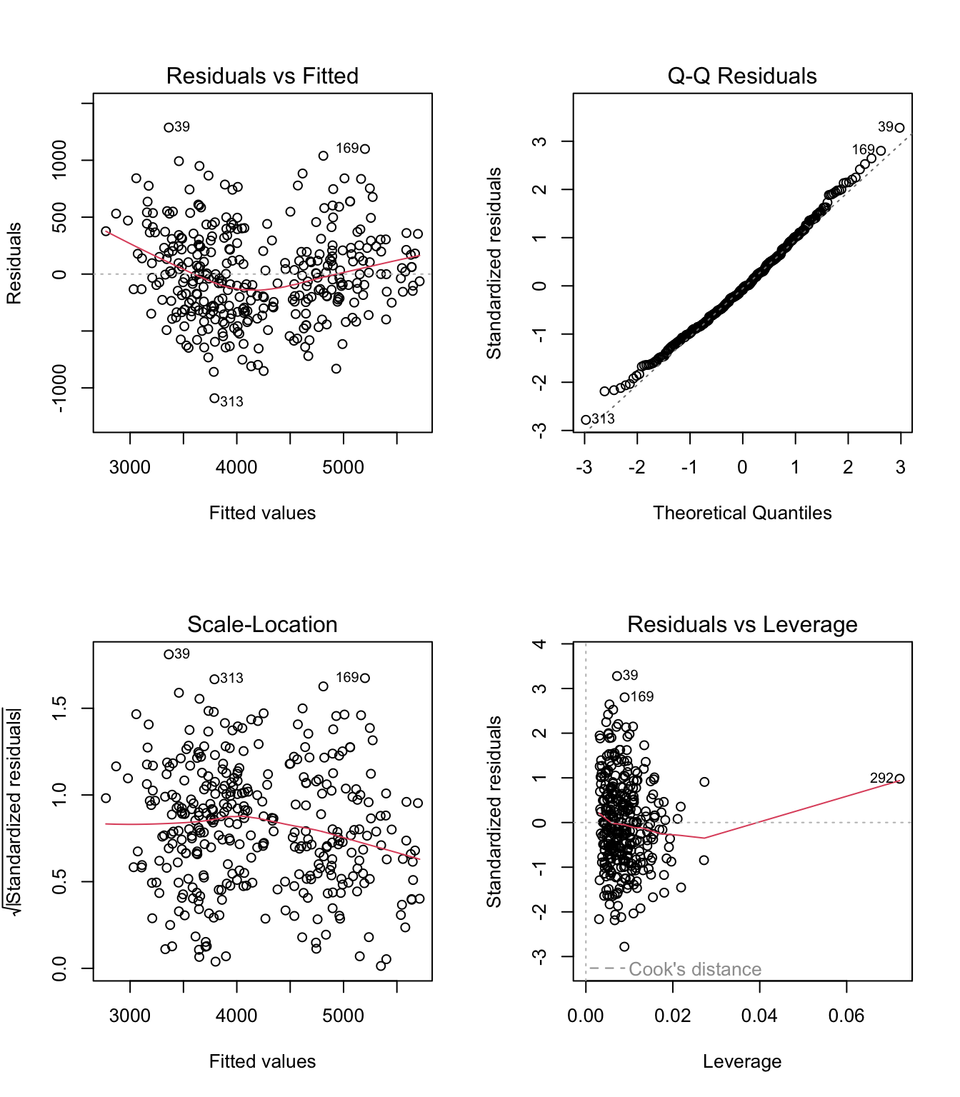
# Fit model for diagnosticspenguins_clean <- penguins |>filter(!is.na(body_mass_g), !is.na(flipper_length_mm), !is.na(bill_length_mm))model2 <-lm(body_mass_g ~ flipper_length_mm + bill_length_mm, data = penguins_clean)# Diagnostic plotspar(mfrow =c(2, 2))plot(model2)
These plots help identify: 1. Residuals vs Fitted: Should show random scatter (linearity, homoscedasticity) 2. Normal Q-Q: Points should follow diagonal line (normality) 3. Scale-Location: Should show random scatter (homoscedasticity) 4. Residuals vs Leverage: Identifies influential outliers
7. Common Mistakes
1. Assuming causation from correlation: Linear regression shows association, not causation. Just because flipper length predicts body mass doesn’t mean longer flippers cause higher mass.
2. Extrapolating beyond data range: Don’t use the model to predict outcomes for predictor values outside your observed range. The linear relationship may not hold.
3. Ignoring assumption violations: Always check diagnostic plots. Violating assumptions can lead to biased estimates, incorrect confidence intervals, and poor predictions.
8. Related Concepts
What to learn next: - Multiple regression: Using categorical predictors, interaction terms - Polynomial regression: Modeling curved relationships - Regularized regression: Ridge and Lasso for high-dimensional data - Logistic regression: For binary outcomes
Alternative methods: - Robust regression: When you have outliers - Generalized linear models: For non-normal outcomes - Random forests or gradient boosting: For complex, non-linear relationships - Mixed-effects models: When you have grouped or nested data
Linear regression serves as the foundation for understanding these more advanced techniques, making it an essential tool in every data scientist’s toolkit.
---title: "How to linear regression basics in R"description: "Linear regression is a fundamental statistical method that models the relationship between a continuous outcome variable (dependent variable) and one or more..."date: 2026-02-21categories: ["statistics", "linear regression basics"]format: html: code-fold: false code-tools: true---## 1. IntroductionLinear regression is a fundamental statistical method that models the relationship between a continuous outcome variable (dependent variable) and one or more predictor variables (independent variables). It assumes this relationship can be represented by a straight line, making it one of the most interpretable machine learning techniques.You would use linear regression when you want to:- Predict a continuous outcome based on other variables- Understand how much each predictor influences the outcome- Test hypotheses about relationships between variables- Create a baseline model for comparison with more complex methodsLinear regression requires several key assumptions:- **Linearity**: The relationship between predictors and outcome is linear- **Independence**: Observations are independent of each other- **Homoscedasticity**: Residuals have constant variance across all fitted values- **Normality**: Residuals are normally distributed- **No multicollinearity**: Predictor variables aren't highly correlated with each otherWhen these assumptions are met, linear regression provides reliable, interpretable results that form the foundation for more advanced statistical modeling techniques.## 2. The MathThe basic linear regression equation is:```Y = β₀ + β₁X₁ + β₂X₂ + ... + βₚXₚ + ε```Where:- **Y** = the outcome variable we're trying to predict- **β₀** = the intercept (value of Y when all X variables equal zero)- **β₁, β₂, βₚ** = coefficients showing how much Y changes for a one-unit increase in each X- **X₁, X₂, Xₚ** = predictor variables- **ε** = error term (residuals - the difference between predicted and actual values)For simple linear regression (one predictor), this simplifies to:```Y = β₀ + β₁X + ε```The goal is to find the best-fitting line by minimizing the sum of squared residuals (ordinary least squares). R calculates these coefficients automatically, but understanding what they represent is crucial for interpretation.## 3. R Implementation```r# Load required packageslibrary(tidyverse)library(palmerpenguins)library(broom)# Load the datadata(penguins)glimpse(penguins)``````Rows: 344Columns: 8$ species <fct> Adelie, Adelie, Adelie, Adelie, Adelie, Adelie, Adel…$ island <fct> Torgersen, Torgersen, Torgersen, Torgersen, Torgerse…$ bill_length_mm <dbl> 39.1, 39.5, 40.3, NA, 36.7, 39.3, 38.9, 39.2, 34.1…$ bill_depth_mm <dbl> 18.7, 17.4, 18.0, NA, 19.3, 20.6, 17.8, 19.6, 18.1…$ flipper_length_mm <int> 181, 186, 195, NA, 193, 190, 181, 195, 193, 190, 18…$ body_mass_g <int> 3750, 3800, 3250, NA, 3450, 3650, 3625, 4675, 3475,…$ sex <fct> male, female, female, NA, female, male, female, male…$ year <int> 2007, 2007, 2007, 2007, 2007, 2007, 2007, 2007, 200…```Basic linear regression in R uses the [`lm()`](simple-linear-regression-in-r.html) function:```r# Simple linear regression: body mass predicted by flipper lengthmodel1 <-lm(body_mass_g ~ flipper_length_mm, data = penguins)summary(model1)``````Call:lm(formula = body_mass_g ~ flipper_length_mm, data = penguins)Residuals: Min 1Q Median 3Q Max -1058.80 -259.27 -26.88 247.33 1288.69 Coefficients: Estimate Std. Error t value Pr(>|t|) (Intercept) -5780.83 305.51 -18.93 <2e-16 ***flipper_length_mm 49.69 1.52 32.72 <2e-16 ***---Signif. codes: 0 '***' 0.001 '**' 0.01 '*' 0.05 '.' 0.1 ' ' 1Residual standard error: 394.3 on 340 degrees of freedom (2 observations deleted due to missingness)Multiple R-squared: 0.759, Adjusted R-squared: 0.7583 F-statistic: 1071 on 1 and 340 DF, p-value: < 2.2e-16```## 4. Full Worked ExampleLet's predict penguin body mass using flipper length and bill length:```r# Remove missing values for clean analysispenguins_clean <- penguins %>%filter(!is.na(body_mass_g), !is.na(flipper_length_mm), !is.na(bill_length_mm))# Multiple linear regressionmodel2 <-lm(body_mass_g ~ flipper_length_mm + bill_length_mm, data = penguins_clean)# Get detailed resultssummary(model2)``````Call:lm(formula = body_mass_g ~ flipper_length_mm + bill_length_mm, data = penguins_clean)Residuals: Min 1Q Median 3Q Max -1003.49 -242.37 -23.98 222.05 1287.42 Coefficients: Estimate Std. Error t value Pr(>|t|) (Intercept) -6787.89 389.00 -17.46 <2e-16 ***flipper_length_mm 45.99 1.73 26.62 <2e-16 ***bill_length_mm 17.33 4.49 3.86 0.000134 ***---Signif. codes: 0 '***' 0.001 '**' 0.01 '*' 0.05 '.' 0.1 ' ' 1Residual standard error: 376.7 on 339 degrees of freedomMultiple R-squared: 0.7739, Adjusted R-squared: 0.7725 F-statistic: 580.4 on 2 and 339 DF, p-value: < 2.2e-16```**Interpreting the results:**- **Intercept (-6787.89)**: The predicted body mass when both flipper length and bill length are zero (not meaningful in this context)- **Flipper length coefficient (45.99)**: For each 1mm increase in flipper length, body mass increases by about 46 grams, holding bill length constant- **Bill length coefficient (17.33)**: For each 1mm increase in bill length, body mass increases by about 17 grams, holding flipper length constant- **R-squared (0.7739)**: About 77% of the variation in body mass is explained by these two predictors- **p-values**: All coefficients are highly significant (p < 0.001)```r# Get confidence intervals for coefficientsconfint(model2)`````` 2.5 % 97.5 %>%(Intercept) -7554.06 -6021.7253flipper_length_mm 42.60 49.3803bill_length_mm 8.52 26.1425```## 5. Visualization```{r}#| message: false#| warning: false# Load packages for visualizationlibrary(tidyverse)library(palmerpenguins)# Prepare clean datapenguins_clean <- penguins |>filter(!is.na(body_mass_g), !is.na(flipper_length_mm))# Scatter plot with regression lineggplot(penguins_clean, aes(x = flipper_length_mm, y = body_mass_g)) +geom_point(aes(color = species), alpha =0.7) +geom_smooth(method ="lm", se =TRUE, color ="black") +labs(title ="Penguin Body Mass vs Flipper Length",subtitle ="Linear regression line with 95% confidence interval",x ="Flipper Length (mm)",y ="Body Mass (g)",color ="Species" ) +theme_minimal() +theme(legend.position ="bottom")```This plot shows the strong positive linear relationship between flipper length and body mass. The gray shaded area represents the 95% confidence interval around the regression line. Different colored points show the three penguin species, revealing that the relationship holds across species, though there are some species-specific patterns.## 6. Assumptions & Limitations**When NOT to use linear regression:**- **Non-linear relationships**: If the relationship curves significantly, consider polynomial regression or other non-linear methods- **Non-constant variance**: If residuals show patterns (fan shapes, curves), you may need data transformation or robust regression- **Highly correlated predictors**: Multicollinearity makes coefficients unstable and hard to interpret**Checking assumptions:**```{r}#| fig-height: 8# Fit model for diagnosticspenguins_clean <- penguins |>filter(!is.na(body_mass_g), !is.na(flipper_length_mm), !is.na(bill_length_mm))model2 <-lm(body_mass_g ~ flipper_length_mm + bill_length_mm, data = penguins_clean)# Diagnostic plotspar(mfrow =c(2, 2))plot(model2)```These plots help identify:1. **Residuals vs Fitted**: Should show random scatter (linearity, homoscedasticity)2. **Normal Q-Q**: Points should follow diagonal line (normality)3. **Scale-Location**: Should show random scatter (homoscedasticity)4. **Residuals vs Leverage**: Identifies influential outliers## 7. Common Mistakes**1. Assuming causation from correlation**: Linear regression shows association, not causation. Just because flipper length predicts body mass doesn't mean longer flippers cause higher mass.**2. Extrapolating beyond data range**: Don't use the model to predict outcomes for predictor values outside your observed range. The linear relationship may not hold.**3. Ignoring assumption violations**: Always check diagnostic plots. Violating assumptions can lead to biased estimates, incorrect confidence intervals, and poor predictions.## 8. Related Concepts**What to learn next:**- **Multiple regression**: Using categorical predictors, interaction terms- **Polynomial regression**: Modeling curved relationships- **Regularized regression**: Ridge and Lasso for high-dimensional data- **Logistic regression**: For binary outcomes**Alternative methods:**- **Robust regression**: When you have outliers- **Generalized linear models**: For non-normal outcomes- **Random forests or gradient boosting**: For complex, non-linear relationships- **Mixed-effects models**: When you have grouped or nested dataLinear regression serves as the foundation for understanding these more advanced techniques, making it an essential tool in every data scientist's toolkit.## Related Tutorials- [Linear Regression in R with lm() function - A Practical Tutorial](simple-linear-regression-in-r.html)- [How to Spearman correlation in R](how-to-spearman-correlation-in-r.html)- [How to Extract p-values from multiple simple linear regression models](extract-p-values-from-multiple-simple-linear-regression-models.html)- [How to perform multiple t-tests using tidyverse](how-to-perform-multiple-t-tests-using-tidyverse.html)- [How to ANOVA two-way in R](how-to-anova-two-way-in-r.html)