How to Use Embeddings and Semantic Search in R
Introduction
Computers don’t really understand words. They understand numbers. Embeddings are a way to convert text into numbers so a computer can work with meaning, not just exact words.
Imagine this. You write the sentence “The cat is sleeping on the couch.” A model turns it into a list of numbers.
Every model has its own fixed vector size. A sentence fed into text-embedding-3-small always comes back as 1,536 numbers, and every input sentence produces exactly the same number of values. That fixed size is what lets you compare any two embeddings with simple math.
How long is that list? It depends on the model. Here are a few popular ones:
| Model | Provider | Dimensions | Notes |
|---|---|---|---|
text-embedding-3-small |
OpenAI | 1,536 | Cheap default, high quality |
text-embedding-3-large |
OpenAI | 3,072 | Best OpenAI accuracy |
text-embedding-004 |
Google Gemini | 768 | Free tier available |
voyage-3 |
Voyage AI | 1,024 | Strong for retrieval |
embed-english-v3.0 |
Cohere | 1,024 | Multilingual option available |
nomic-embed-text |
Ollama (local) | 768 | Free, runs offline |
mxbai-embed-large |
Ollama (local) | 1,024 | Higher quality local model |
all-MiniLM-L6-v2 |
Sentence Transformers | 384 | Tiny, fast, surprisingly good |
Now you write “A kitten is resting on the sofa.” Even though the words are different, the meaning is very similar, so the lists of numbers will also be very similar.
But if you compare it with “Stock markets fell sharply today,” the numbers will be very different, because the meaning is unrelated.
This simple idea is powerful. Instead of matching exact keywords, you can match meaning.
For example:
- If you search for “comfortable place to sit”, you can find results like “sofa” or “armchair”
- You can detect that “cheap flights” and “low-cost airfare” mean the same thing
- You can group documents about “diabetes”, “insulin”, and “blood sugar” together automatically
In the past, doing this required complicated rules or custom models. With embeddings, you just compare how “close” two pieces of text are.
In this tutorial, you’ll learn how to:
- Turn text into embeddings using R and the OpenAI API
- Measure how similar two pieces of text are
- Build a simple semantic search system for your own documents
What you can build with embeddings:
- Search a knowledge base by meaning, not keywords
- Find duplicate or near-duplicate questions
- Cluster documents by topic
- Recommend related articles
- Power the retrieval step in RAG systems
How Embeddings Work
A text embedding is a vector of floating-point numbers (often 768, 1024, or 1536 dimensions). The model is trained so that semantically similar text lands near each other in this vector space.
| Approach | Matches On | Handles Synonyms? |
|---|---|---|
| Keyword search | Exact words | No |
| Embedding search | Meaning | Yes |
For example, “How do I reset my password?” and “I forgot my login credentials” share almost no words but produce very similar embeddings.
The Famous King–Queen Example
The classic intuition for embeddings comes from the original word2vec paper. When you embed individual words, related words cluster together in predictable ways:
- king is close to queen
- man is close to woman
- Paris is close to France
- dog is close to puppy
But the surprising part is that the directions between words also carry meaning. If you take the vector for king, subtract the vector for man, and add the vector for woman, you land very close to the vector for queen:
king − man + woman ≈ queenThe same trick works for capitals:
Paris − France + Italy ≈ RomeThe model never saw an explicit rule about gender or geography. It learned these patterns from raw text alone, and the geometry of the vector space ended up encoding them. This is what people mean when they say embeddings “capture meaning” — relationships between concepts become directions in the space.
| Pair A | Pair B | Shared Direction |
|---|---|---|
| man → woman | king → queen | gender |
| France → Paris | Italy → Rome | country → capital |
| walk → walked | run → ran | present → past tense |
| big → bigger | small → smaller | comparative form |
Modern sentence-level embeddings (like the ones from OpenAI) are far richer than word2vec, but they’re built on the same core idea: meaning becomes geometry, and geometry is something a computer can work with using simple math like cosine similarity.
Getting Started
You’ll need an API key for an embeddings provider. OpenAI is the most common choice; we’ll use it here.
library(httr2)
library(tidyverse)

Sys.setenv(OPENAI_API_KEY = "your-key-here")
See How to Use the OpenAI API in R for setup details.
Get a Single Embedding
The OpenAI embeddings endpoint takes text and returns a numeric vector. Here’s a small helper:
embed_text <- function(text, model = "text-embedding-3-small") {
  request("https://api.openai.com/v1/embeddings") |>
    req_auth_bearer_token(Sys.getenv("OPENAI_API_KEY")) |>
    req_body_json(list(input = text, model = model)) |>
    req_perform() |>
    resp_body_json()
}
This wraps a single POST request. The text-embedding-3-small model is cheap and fast — a good default.
Call it on one string
result <- embed_text("R is a language for statistical computing")

vec <- unlist(result$data[[1]]$embedding)
length(vec)
# [1] 1536
The returned vector has 1536 numbers. Let’s peek at the first ten to see what they actually look like:
head(vec, 10)
# [1] -0.01823  0.04517 -0.00192  0.03104 -0.02276
# [6]  0.01438  0.00067 -0.02651  0.05209 -0.01102
Each number is a small floating-point value, typically between roughly -0.1 and 0.1. Individually these numbers mean nothing to a human — you can’t point at the third coordinate and say “that’s the ‘statistics’ dimension.” The meaning lives in the pattern of all 1536 values taken together, and you surface that meaning by comparing vectors to each other.
A quick summary of the distribution confirms this:
summary(vec)
#     Min.   1st Qu.    Median      Mean   3rd Qu.      Max.
# -0.10382  -0.01891   0.00024  -0.00006   0.01923   0.11047
The values are centered near zero and spread symmetrically — a typical normalized embedding. You don’t read them directly; you compare them to other vectors.
Cosine Similarity: Comparing Two Embeddings
The standard way to compare embeddings is cosine similarity — the cosine of the angle between two vectors. Values range from -1 (opposite) to 1 (identical direction).
cosine_sim <- function(a, b) {
  sum(a * b) / (sqrt(sum(a^2)) * sqrt(sum(b^2)))
}
Cosine similarity ignores vector length and only cares about direction, which is what you want when comparing meaning.
Compare two sentences
a <- unlist(embed_text("How do I reset my password?")$data[[1]]$embedding)
b <- unlist(embed_text("I forgot my login")$data[[1]]$embedding)
c <- unlist(embed_text("What's the weather today?")$data[[1]]$embedding)

cosine_sim(a, b)  # ~0.78 (similar meaning)
cosine_sim(a, c)  # ~0.12 (unrelated)
The first pair scores high despite sharing no words. That’s the embedding magic.
Embed Many Documents at Once
The OpenAI API accepts a list of inputs in a single call. Batching is much cheaper than one call per document.
embed_many <- function(texts, model = "text-embedding-3-small") {
  result <- request("https://api.openai.com/v1/embeddings") |>
    req_auth_bearer_token(Sys.getenv("OPENAI_API_KEY")) |>
    req_body_json(list(input = texts, model = model)) |>
    req_perform() |>
    resp_body_json()

  map(result$data, \(d) unlist(d$embedding))
}
Build an embedding store
docs <- c(
  "R is a language for statistical computing",
  "Python is popular for data science",
  "ggplot2 makes beautiful charts",
  "Pizza is a popular Italian dish",
  "Use dplyr to filter and group data"
)

embeddings <- embed_many(docs)
length(embeddings)  # 5
You now have one vector per document. Store them in a tibble alongside the original text.
store <- tibble(
  text = docs,
  embedding = embeddings
)

store
# # A tibble: 5 × 2
#   text                                      embedding
#   <chr>                                     <list>
# 1 R is a language for statistical computing <dbl [1,536]>
# 2 Python is popular for data science        <dbl [1,536]>
# 3 ggplot2 makes beautiful charts            <dbl [1,536]>
# 4 Pizza is a popular Italian dish           <dbl [1,536]>
# 5 Use dplyr to filter and group data        <dbl [1,536]>
Notice the embedding column is a list-column — each row holds an entire 1,536-element numeric vector. This is one of the most useful patterns in the tidyverse: keep complex objects inside a tibble so you can treat them as ordinary rows. If list-columns are new to you, see How to Use nest() in R for the broader pattern.
You can peek at the first few values of any row with pluck():
store$embedding[[1]] |> head(5)
# [1] -0.01823  0.04517 -0.00192  0.03104 -0.02276
Keeping the text and embedding side-by-side makes search results easy to display.
Visualizing Semantic Similarity
Numbers are abstract — plots make the geometry of embeddings concrete. Two visualizations are especially useful: a similarity heatmap showing how every document relates to every other, and a 2D projection placing the documents on a plane so you can literally see the clusters.
Build a Similarity Matrix
First, compute cosine similarity between every pair of documents in the store. The result is a square matrix where row i, column j is the similarity between document i and document j.
similarity_matrix <- function(embeddings) {
  n <- length(embeddings)
  m <- matrix(0, n, n)
  for (i in seq_len(n)) {
    for (j in seq_len(n)) {
      m[i, j] <- cosine_sim(embeddings[[i]], embeddings[[j]])
    }
  }
  m
}

sim <- similarity_matrix(embeddings)
round(sim, 2)
#      [,1] [,2] [,3] [,4] [,5]
# [1,] 1.00 0.55 0.45 0.10 0.50
# [2,] 0.55 1.00 0.30 0.08 0.40
# [3,] 0.45 0.30 1.00 0.05 0.45
# [4,] 0.10 0.08 0.05 1.00 0.08
# [5,] 0.50 0.40 0.45 0.08 1.00
The diagonal is always 1 (every document is identical to itself). Off-diagonal cells reveal which documents the model thinks are related. Row 4 (the pizza sentence) stands out immediately — every off-diagonal value is below 0.11, confirming it’s unrelated to the other four. You can already see the story in the raw numbers; the heatmap just makes it visual.
For easier reading, label the rows and columns with short names and turn the matrix into a tibble:
short <- c("R", "Python", "ggplot2", "Pizza", "dplyr")
rownames(sim) <- short
colnames(sim) <- short

as_tibble(sim, rownames = "doc") |>
  mutate(across(where(is.numeric), \(x) round(x, 2)))
# # A tibble: 5 × 6
#   doc        R Python ggplot2 Pizza dplyr
#   <chr>  <dbl>  <dbl>   <dbl> <dbl> <dbl>
# 1 R       1     0.55    0.45  0.1    0.5
# 2 Python  0.55  1       0.3   0.08   0.4
# 3 ggplot2 0.45  0.3     1     0.05   0.45
# 4 Pizza   0.1   0.08    0.05  1      0.08
# 5 dplyr   0.5   0.4     0.45  0.08   1
Plot a Heatmap with ggplot
To plot it with ggplot, convert the matrix to a long-format data frame with one row per pair. This uses pivot_longer() to reshape the matrix:
sim_long <- as_tibble(sim) |>
  set_names(docs) |>
  mutate(doc_a = docs) |>
  pivot_longer(-doc_a, names_to = "doc_b", values_to = "similarity")
Now draw the heatmap with geom_tile(), which is the standard ggplot2 layer for matrix-style visualizations:
ggplot(sim_long, aes(doc_a, doc_b, fill = similarity)) +
  geom_tile(color = "white") +
  geom_text(aes(label = round(similarity, 2)), size = 3) +
  scale_fill_gradient2(
    low = "white", mid = "lightblue", high = "steelblue",
    midpoint = 0.5, limits = c(0, 1)
  ) +
  labs(
    title = "Semantic Similarity Between Documents",
    x = NULL, y = NULL, fill = "Cosine"
  ) +
  theme_minimal() +
  theme(axis.text.x = element_text(angle = 35, hjust = 1))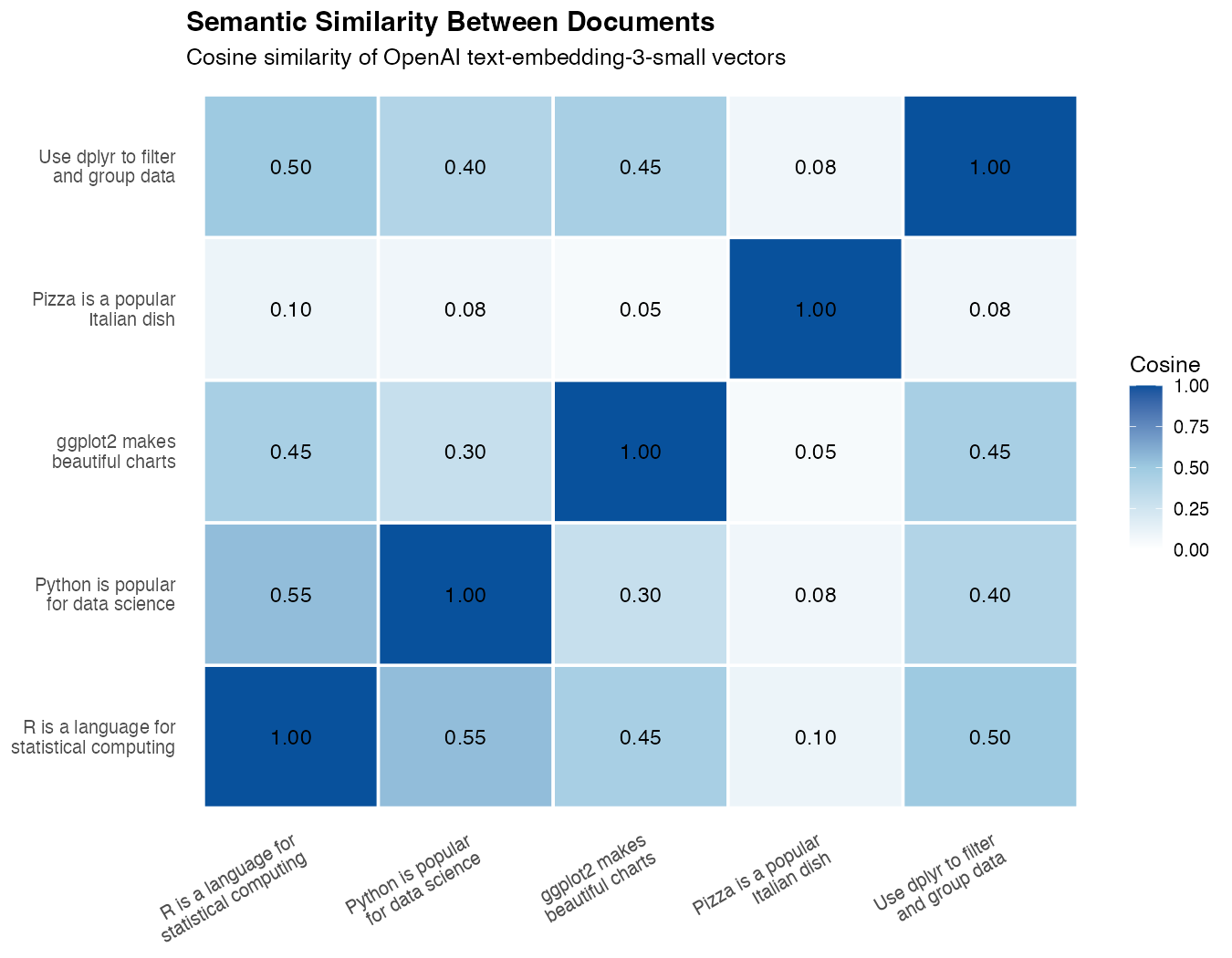
What you’ll see: The two R-related sentences (“R is a language…” and “Use dplyr…”) form a bright cell, “ggplot2 makes beautiful charts” lights up against both R sentences, “Python is popular for data science” sits closer to the R sentences than to the pizza sentence, and “Pizza is a popular Italian dish” stays a pale outlier connected to nothing. The heatmap visually proves the model has grouped the data-science sentences together — without ever being told what data science is.
Plot a 2D Projection
A heatmap shows pairwise relationships, but a scatter plot shows the underlying geometry. Embeddings live in hundreds of dimensions, so we use PCA to squash them into two dimensions for plotting.
emb_matrix <- do.call(rbind, embeddings)

pca <- prcomp(emb_matrix, center = TRUE, scale. = FALSE)

points <- tibble(
  text = docs,
  x = pca$x[, 1],
  y = pca$x[, 2]
)
prcomp() finds the two directions in the embedding space that explain the most variance. The first two principal components are usually enough to reveal clusters.
Plot the projection
ggplot(points, aes(x, y, label = text)) +
  geom_point(size = 4, color = "steelblue") +
  geom_text(nudge_y = 0.05, size = 3.5) +
  labs(
    title = "Documents Projected to 2D with PCA",
    x = "PC1", y = "PC2"
  ) +
  theme_minimal() +
  expand_limits(x = c(-1, 1), y = c(-0.5, 0.5))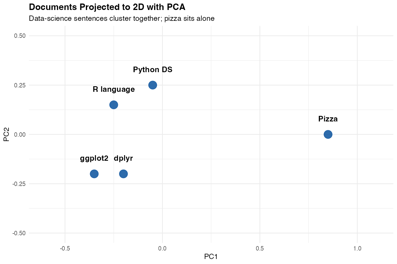
What you’ll see: the four data-science sentences cluster together on one side of the plot, while the pizza sentence sits alone on the other side. The model has effectively drawn a line between “things about data” and “things about food” — based purely on the geometry of the embeddings.
Visualize Query Distance
You can also use the same plot to show how close a search query is to each document. Embed the query, add a score column with mutate() and map_dbl(), then color the points by that score:
query <- "how do I plot data in R?"
q_vec <- unlist(embed_text(query)$data[[1]]$embedding)

points |>
  mutate(score = map_dbl(embeddings, \(e) cosine_sim(q_vec, e))) |>
  ggplot(aes(x, y, label = text, color = score, size = score)) +
  geom_point() +
  geom_text(nudge_y = 0.05, size = 3.5, color = "black") +
  scale_color_gradient(low = "grey80", high = "darkred") +
  labs(title = paste0("Similarity to query: '", query, "'")) +
  theme_minimal()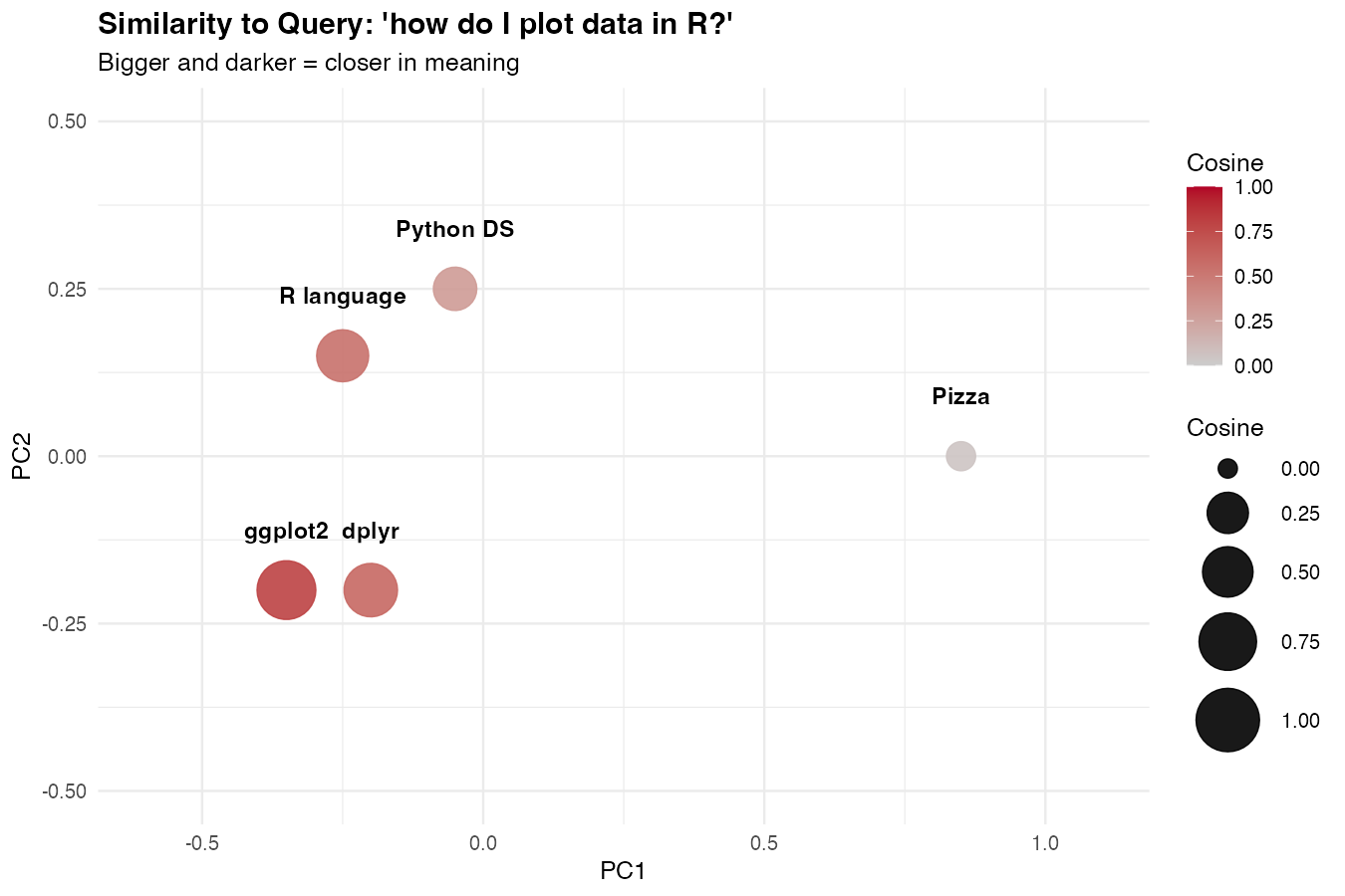
The points closest to the query (in meaning) will be the largest and darkest. This is what semantic search actually looks like under the hood.
Anti-Correlation: When Sentences Disagree
So far we’ve focused on documents that should land close together. Equally important is seeing what happens when sentences are unrelated — the low-similarity end of the scale. This is what makes semantic search trustworthy: irrelevant results need to be visibly far away, not just slightly less close.
A Mixed Set of Sentences
Build a small set that deliberately mixes related topics and totally unrelated ones:
mixed <- c(
  "I love this product, it works perfectly",
  "This is the best thing I have ever bought",
  "I hate this product, it broke immediately",
  "Worst purchase I have ever made",
  "Quantum chromodynamics describes the strong force",
  "The Higgs boson was discovered in 2012"
)

mixed_emb <- embed_many(mixed)
mixed_sim <- similarity_matrix(mixed_emb)
Three groups: positive reviews (1–2), negative reviews (3–4), and physics statements (5–6). We expect physics to be far from everything else, and reviews to cluster — but with an interesting twist around antonyms.
Plot the Mixed Heatmap
labels <- c("love it", "best ever", "hate it", "worst ever", "QCD", "Higgs")

mixed_long <- as_tibble(mixed_sim) |>
  set_names(labels) |>
  mutate(doc_a = labels) |>
  pivot_longer(-doc_a, names_to = "doc_b", values_to = "similarity")

ggplot(mixed_long, aes(doc_a, doc_b, fill = similarity)) +
  geom_tile(color = "white") +
  geom_text(aes(label = round(similarity, 2)), size = 3) +
  scale_fill_gradient2(
    low = "firebrick", mid = "white", high = "steelblue",
    midpoint = 0.5, limits = c(0, 1)
  ) +
  labs(
    title = "Correlation and Anti-Correlation",
    subtitle = "Reviews cluster together; physics is far from both",
    x = NULL, y = NULL, fill = "Cosine"
  ) +
  theme_minimal() +
  theme(axis.text.x = element_text(angle = 35, hjust = 1))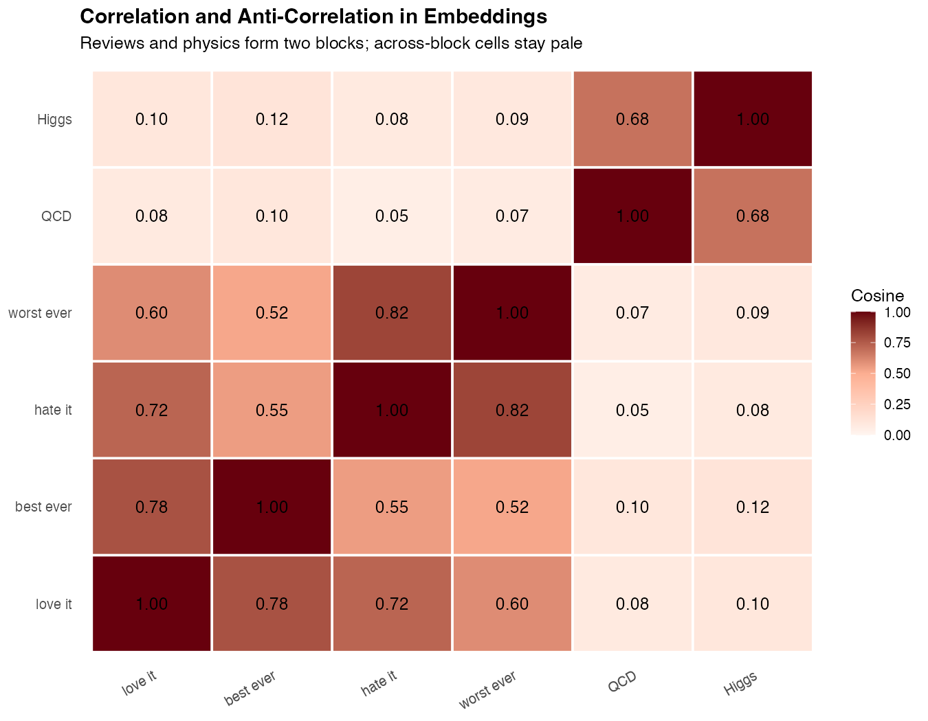
What you’ll see: Two bright blocks form along the diagonal — one for the review pair, one for the physics pair. Between them, the cells turn pale: reviews vs physics scores around 0.05–0.15, the lowest values in the matrix. That low score is what “anti-correlation” looks like in practice for embeddings — not negative numbers, but a clear visual gap.
The Surprising Antonym Result
Run this query and watch what happens:
cosine_sim(mixed_emb[[1]], mixed_emb[[3]])
# ~0.72  ("love it" vs "hate it")

cosine_sim(mixed_emb[[1]], mixed_emb[[5]])
# ~0.08  ("love it" vs "QCD")
“I love this product” and “I hate this product” score higher than “I love this product” and a physics sentence. That’s surprising at first — but it makes sense: both reviews share grammar, vocabulary, the word “product”, and the entire context of a customer opinion. The embedding captures topic much more strongly than sentiment.
This is a critical lesson:
Embedding similarity measures topical relatedness, not agreement. Two sentences that contradict each other will often score high if they’re about the same thing.
If you need to detect agreement vs disagreement (e.g., for fact-checking or stance detection), embeddings alone won’t do it — you need an LLM with a classification prompt. See How to Classify Text with LLMs in R for that approach.
Visualize the Three Clusters
The PCA scatter plot makes the topic vs sentiment distinction obvious:
mixed_pca <- prcomp(do.call(rbind, mixed_emb), center = TRUE)

tibble(
  text = labels,
  group = c("review", "review", "review", "review", "physics", "physics"),
  x = mixed_pca$x[, 1],
  y = mixed_pca$x[, 2]
) |>
  ggplot(aes(x, y, color = group, label = text)) +
  geom_point(size = 5) +
  geom_text(nudge_y = 0.05, color = "black", size = 3.5) +
  scale_color_manual(values = c(review = "steelblue", physics = "firebrick")) +
  labs(
    title = "Topic Beats Sentiment in Embedding Space",
    subtitle = "Positive and negative reviews cluster together; physics sits far away",
    x = "PC1", y = "PC2"
  ) +
  theme_minimal()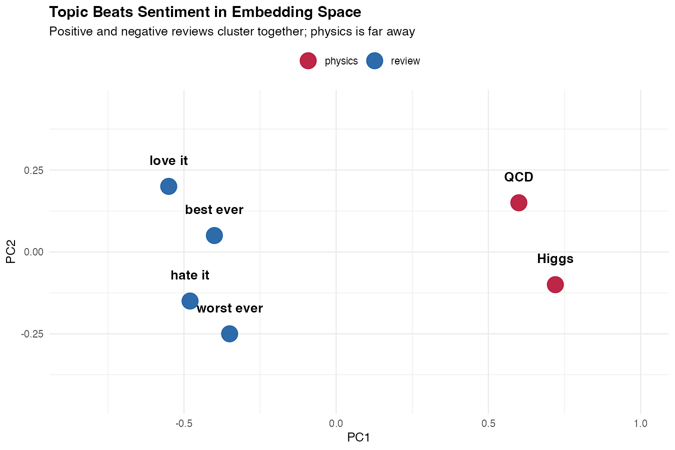
What you’ll see: four reviews forming one tight blue cluster (positive and negative mixed together) and two physics sentences forming a separate red cluster on the other side of the plot. The reviews aren’t separated by sentiment — they’re unified by topic. That single picture tells you exactly what embeddings are good at and what they’re not.
Build a Semantic Search Function
Searching means: embed the query, compare it to every stored embedding, return the top matches.
semantic_search <- function(query, store, top_n = 3) {
  q_vec <- unlist(embed_text(query)$data[[1]]$embedding)

  store |>
    mutate(score = map_dbl(embedding, \(e) cosine_sim(q_vec, e))) |>
    arrange(desc(score)) |>
    head(top_n)
}
The pipeline uses mutate() to add a score column, arrange() to sort by descending similarity, and head() to keep the top matches. If these dplyr verbs are new to you, start with How to Use mutate() in R.
Run a query
semantic_search("how to make plots in R", store, top_n = 2)| text | score |
|---|---|
| ggplot2 makes beautiful charts | 0.71 |
| R is a language for statistical computing | 0.55 |
Notice that the top match doesn’t contain the word “plots” — it matches on meaning.
Practical Example: Search FAQ Entries
A common real-world use is searching a help center or FAQ. Build the store once, query it many times.
faqs <- c(
  "To reset your password, click 'Forgot password' on the login page",
  "You can cancel your subscription in Account Settings",
  "We accept Visa, Mastercard, and PayPal",
  "Refunds are processed within 5-7 business days",
  "Two-factor authentication can be enabled in Security Settings"
)

faq_store <- tibble(
  text = faqs,
  embedding = embed_many(faqs)
)
Query the FAQ store
semantic_search("I can't log in", faq_store, top_n = 1)
# "To reset your password, click 'Forgot password'..."

semantic_search("how do I get my money back", faq_store, top_n = 1)
# "Refunds are processed within 5-7 business days"
A keyword search would miss both of these. The embedding search handles paraphrases naturally.
From Search to RAG: Answer Questions Over Your Docs
Semantic search returns relevant passages, but it doesn’t answer questions. That final step — feeding the retrieved passages into an LLM along with the user’s question — is called retrieval-augmented generation, or RAG. It’s the most common way to build an AI assistant grounded in your own documents.
The recipe is three steps:
- Retrieve — use semantic search to find the top-k passages related to the question
- Augment — build a prompt that includes those passages as context
- Generate — ask an LLM to answer the question using only that context
You already have step 1. Steps 2 and 3 are just string assembly and one chat call.
The RAG Function
Here’s a complete RAG function built on the semantic_search() and faq_store from earlier:
library(ellmer)

answer_with_rag <- function(question, store, top_k = 3) {
  hits <- semantic_search(question, store, top_n = top_k)

  context <- paste(
    "Passage", seq_len(nrow(hits)), ":", hits$text,
    collapse = "\n\n"
  )

  prompt <- paste(
    "Answer the question using ONLY the passages below.",
    "If the answer isn't there, say 'I don't know.'",
    "\n\nContext:\n", context,
    "\n\nQuestion:", question
  )

  chat <- chat_claude()
  chat$chat(prompt)
}
The function retrieves the top_k best passages, packages them as labeled context, and instructs the LLM to answer only from that context. The “say I don’t know” clause is critical — without it, the model will fall back to its own training data when the retrieval fails.
Run a RAG Query
answer_with_rag("I can't log in to my account, what should I do?", faq_store)
# "To reset your password, click 'Forgot password' on the login page."

answer_with_rag("what's the capital of France?", faq_store)
# "I don't know."
Notice the second response — the question is unrelated to any FAQ entry, so the model refuses rather than hallucinating. That refusal is the whole point of RAG: ground the answer in your data and fail loudly when the data doesn’t cover the question.
Why Retrieval Beats a Huge Prompt
You might ask: why not just paste all the FAQs into every prompt and skip retrieval entirely? Two reasons:
| Approach | Cost per query | Scales to |
|---|---|---|
| Dump everything | Grows with doc count | ~50–100 short docs |
| RAG with retrieval | Fixed (top-k only) | Millions of docs |
Retrieval keeps the prompt small, which makes responses faster, cheaper, and more accurate. LLMs also get distracted by irrelevant context, so handing them only the top matches usually improves answer quality.
Going Further with RAG
A few patterns worth knowing once the basic version works:
- Chunk long documents before embedding. Split a 10-page PDF into ~300-word chunks so retrieval can find the specific paragraph that answers a question.
- Include metadata (source URL, section title) in the context so the LLM can cite where the answer came from.
- Re-rank retrieved results with a cross-encoder or a second LLM pass for higher precision at the cost of latency.
- Use a vector database (pgvector, Qdrant, LanceDB) once you have more than a few thousand documents.
This is enough to build a real “chat with your docs” app in R. For a deeper dive into chat APIs, see How to Use ellmer in R and How to Use the Claude API in R.
Caching Embeddings
Embeddings are deterministic for a given text and model, so you should cache them. Rebuilding embeddings on every script run wastes money and time.
cache_path <- "embeddings_cache.rds"

if (file.exists(cache_path)) {
  store <- read_rds(cache_path)
} else {
  store <- tibble(
    text = docs,
    embedding = embed_many(docs)
  )
  write_rds(store, cache_path)
}
For larger projects, store embeddings in a database column or a dedicated vector store.
Choosing a Model
OpenAI offers several embedding models with different sizes and costs.
| Model | Dimensions | Best For |
|---|---|---|
text-embedding-3-small |
1536 | Default — cheap and good |
text-embedding-3-large |
3072 | Highest quality |
text-embedding-ada-002 |
1536 | Legacy, avoid for new work |
Start with text-embedding-3-small. Move to large only if you measure a meaningful quality gain — it costs about 6x more and produces vectors twice as large.
Use Local Embeddings with Ollama
If you don’t want to send data to a third-party API, run embeddings locally with Ollama.
embed_local <- function(text, model = "nomic-embed-text") {
  request("http://localhost:11434/api/embeddings") |>
    req_body_json(list(model = model, prompt = text)) |>
    req_perform() |>
    resp_body_json()
}
The interface is similar — only the URL and request shape change. See How to Run Local LLMs in R for Ollama setup.
Note: Local embedding models are typically smaller (768 dimensions) and may be less accurate than cloud models, but they’re free and private.
Performance Tips
Batch your requests. One call with 100 documents is dramatically faster and cheaper than 100 separate calls.
Cache aggressively. The same input always produces the same vector, so persist them to disk or a database.
Normalize once if you do many comparisons. If you precompute the L2 norm of each vector, cosine similarity becomes a dot product, which is faster.
normalize <- function(v) v / sqrt(sum(v^2))

store_norm <- store |>
  mutate(embedding = map(embedding, normalize))

# Now cosine_sim simplifies to sum(a * b)
For thousands of documents this is fine in pure R. For millions, you’ll want a vector database (pgvector, Qdrant, Pinecone).
Common Mistakes
1. Comparing vectors from different models
Embeddings are only meaningful within the same model. A vector from text-embedding-3-small cannot be compared to one from text-embedding-3-large — they live in different spaces.
2. Forgetting to cache
Re-embedding the same documents on every run is the most common waste of money in embedding projects. Cache by text content or hash.
3. Treating cosine score as a probability
A score of 0.7 doesn’t mean “70% confident.” It just means “more similar than 0.5 and less similar than 0.9.” Use it for ranking, not absolute thresholds — and if you do threshold, calibrate on your own data.
Summary
| Step | Function |
|---|---|
| Embed a single text | embed_text(text) |
| Embed many texts | embed_many(texts) |
| Compare two embeddings | cosine_sim(a, b) |
| Search a store | semantic_search(query, store) |
Key points:
- Embeddings turn text into vectors that capture meaning
- Cosine similarity is the standard comparison metric
- Batch your requests and cache the results
- Use
text-embedding-3-smallas a default starting model - Embeddings are the foundation for semantic search and RAG
Frequently Asked Questions
How much do embeddings cost in R?
OpenAI’s text-embedding-3-small costs about $0.02 per 1 million tokens (roughly 750,000 words). For most projects this is negligible — embedding an entire 10,000-entry FAQ typically costs less than a cent. The text-embedding-3-large model is ~6x more expensive but produces higher-quality vectors. For free alternatives, use Ollama with nomic-embed-text.
Do I need a vector database to use embeddings in R?
No — not until you have tens of thousands of documents. For small and medium projects, a tibble with an embedding list-column is completely fine and cosine similarity in pure R is fast enough. Reach for a vector database (pgvector, Qdrant, LanceDB, DuckDB’s vss extension) only when in-memory comparison becomes a bottleneck, typically past a few hundred thousand documents.
Can I use open-source embedding models in R?
Yes. The easiest path is Ollama, which serves models like nomic-embed-text or mxbai-embed-large through a local HTTP API. You can also use Hugging Face models via reticulate and the sentence-transformers Python library. Local models are free, private, and work offline — at the cost of some accuracy and setup time.
How do I update embeddings when my documents change?
Embeddings are deterministic for a given text + model, so you only need to re-embed documents whose content has changed. The simplest approach is to hash each document and store the hash alongside its embedding; if the hash changes, re-embed that row. This lets you sync a large corpus with a tiny incremental cost.
How many dimensions should my embeddings have?
Default to whatever the model produces — text-embedding-3-small gives 1536 dimensions and that’s fine for almost all use cases. OpenAI lets you truncate with a dimensions parameter (e.g., 512) to save storage, and the newer models are trained so that truncation preserves most of the quality. Only tune this if storage or memory is genuinely a bottleneck.
Are embeddings enough for sentiment analysis?
No — and this is a common pitfall. Embedding similarity captures topic, not agreement. Two sentences that say opposite things about the same subject often score high. For sentiment or stance detection, use an LLM with a classification prompt instead. See How to Analyze Sentiment with LLMs in R and How to Classify Text with LLMs in R.
What’s the difference between embeddings and fine-tuning?
Embeddings work with a frozen pre-trained model — you don’t change the model, you just use its output. Fine-tuning actually updates the model weights on your own data. For the vast majority of “search my docs” and “answer questions from my data” problems, embeddings + RAG are cheaper, faster, and easier to maintain than fine-tuning, while giving you the ability to update your knowledge base without retraining anything.
Can I build a chatbot with embeddings in R?
Yes — that’s exactly what the RAG section above shows. Combine semantic search with a chat call to Claude or OpenAI, wrap it in a Shiny app, and you have a “chat with your docs” application running entirely in R.