How to use geom_point() in R
Introduction
The geom_point() function is one of the most fundamental geometric objects in ggplot2, used to create scatter plots by adding points to a plot. This function is essential for visualizing relationships between two continuous variables, identifying patterns, outliers, and correlations in your data. It’s particularly useful in exploratory data analysis, allowing you to quickly assess the distribution and relationship of variables. The function comes from the ggplot2 package, which is part of the tidyverse ecosystem. Whether you’re examining the relationship between penguin bill length and depth, car weight and fuel efficiency, or any other paired variables, geom_point() provides a clear, intuitive way to visualize these relationships with extensive customization options.
Syntax
geom_point(
  mapping = NULL,
  data = NULL,
  stat = "identity",
  position = "identity",
  ...,
  na.rm = FALSE,
  show.legend = NA,
  inherit.aes = TRUE
)
Key Arguments: - mapping: Aesthetic mappings (x, y, color, size, shape, alpha) - data: Dataset to use (inherits from ggplot() if not specified) - size: Size of points (numeric value or mapped to variable) - color/colour: Color of points (string or mapped to variable) - shape: Shape of points (numeric 0-25 or mapped to variable) - alpha: Transparency level (0-1) - na.rm: Remove missing values (TRUE/FALSE)
Example 1: Basic Usage
library(tidyverse)
library(palmerpenguins)

# Basic scatter plot
ggplot(penguins, aes(x = bill_length_mm, y = bill_depth_mm)) +
  geom_point(na.rm = TRUE) +
  labs(
    title = "Penguin Bill Length vs Bill Depth",
    x = "Bill Length (mm)",
    y = "Bill Depth (mm)"
  )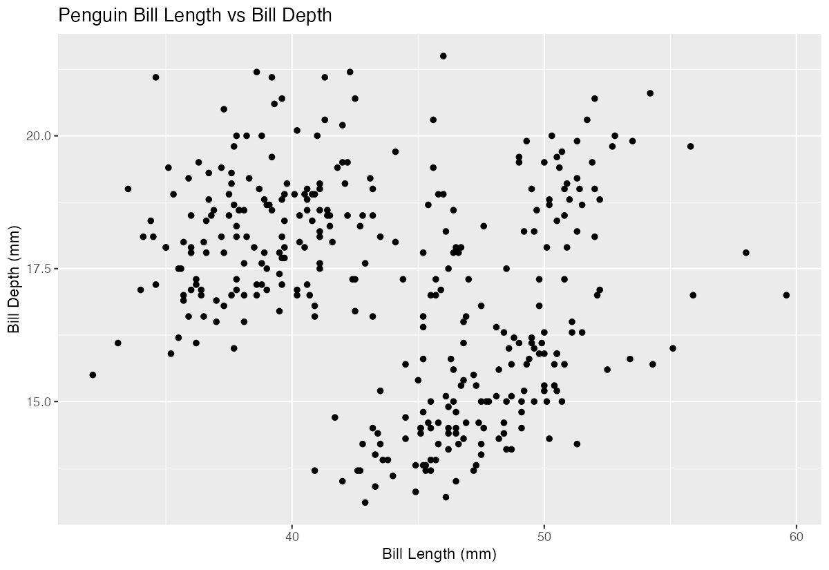
This creates a simple scatter plot showing the relationship between penguin bill length and bill depth. Each point represents one penguin, with bill length on the x-axis and bill depth on the y-axis. The plot reveals interesting patterns in the data, suggesting there might be distinct groups or species with different bill characteristics. The geom_point() function automatically handles the positioning of points based on their x and y coordinates.
Example 2: Practical Application
# Enhanced scatter plot with species mapping and customization
penguins |>
  filter(!is.na(bill_length_mm), !is.na(bill_depth_mm)) |>
  ggplot(aes(x = bill_length_mm, y = bill_depth_mm)) +
  geom_point(aes(color = species, size = body_mass_g), alpha = 0.7) +
  scale_color_viridis_d(name = "Species") +
  scale_size_continuous(name = "Body Mass (g)", range = c(2, 6)) +
  labs(
    title = "Penguin Bill Dimensions by Species",
    x = "Bill Length (mm)",
    y = "Bill Depth (mm)",
    caption = "Data from Palmer Archipelago LTER"
  ) +
  theme_minimal()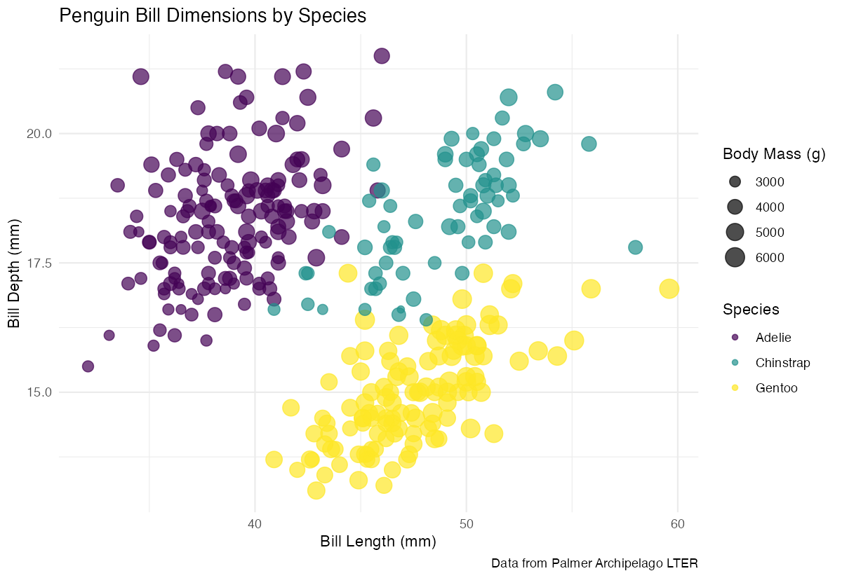
This practical example demonstrates how geom_point() can reveal complex relationships in data. By mapping species to color and body mass to size, we create a multi-dimensional visualization. The alpha = 0.7 parameter adds transparency to handle overlapping points, while the viridis color scale ensures accessibility. This approach is common in scientific publications and business analytics where multiple variables need to be compared simultaneously.
Example 3: Advanced Usage
# Advanced customization with faceting and custom shapes
penguins |>
  filter(!is.na(sex)) |>
  ggplot(aes(x = flipper_length_mm, y = body_mass_g)) +
  geom_point(
    aes(shape = species, color = island),
    size = 3,
    alpha = 0.8,
    stroke = 1.5
  ) +
  facet_wrap(~ sex) +
  scale_shape_manual(values = c(16, 17, 18)) +
  scale_color_brewer(type = "qual", palette = "Set2") +
  labs(
    title = "Flipper Length vs Body Mass by Sex, Species, and Island",
    x = "Flipper Length (mm)",
    y = "Body Mass (g)"
  ) +
  theme_bw() +
  theme(
    strip.background = element_rect(fill = "lightgray"),
    legend.position = "bottom"
  )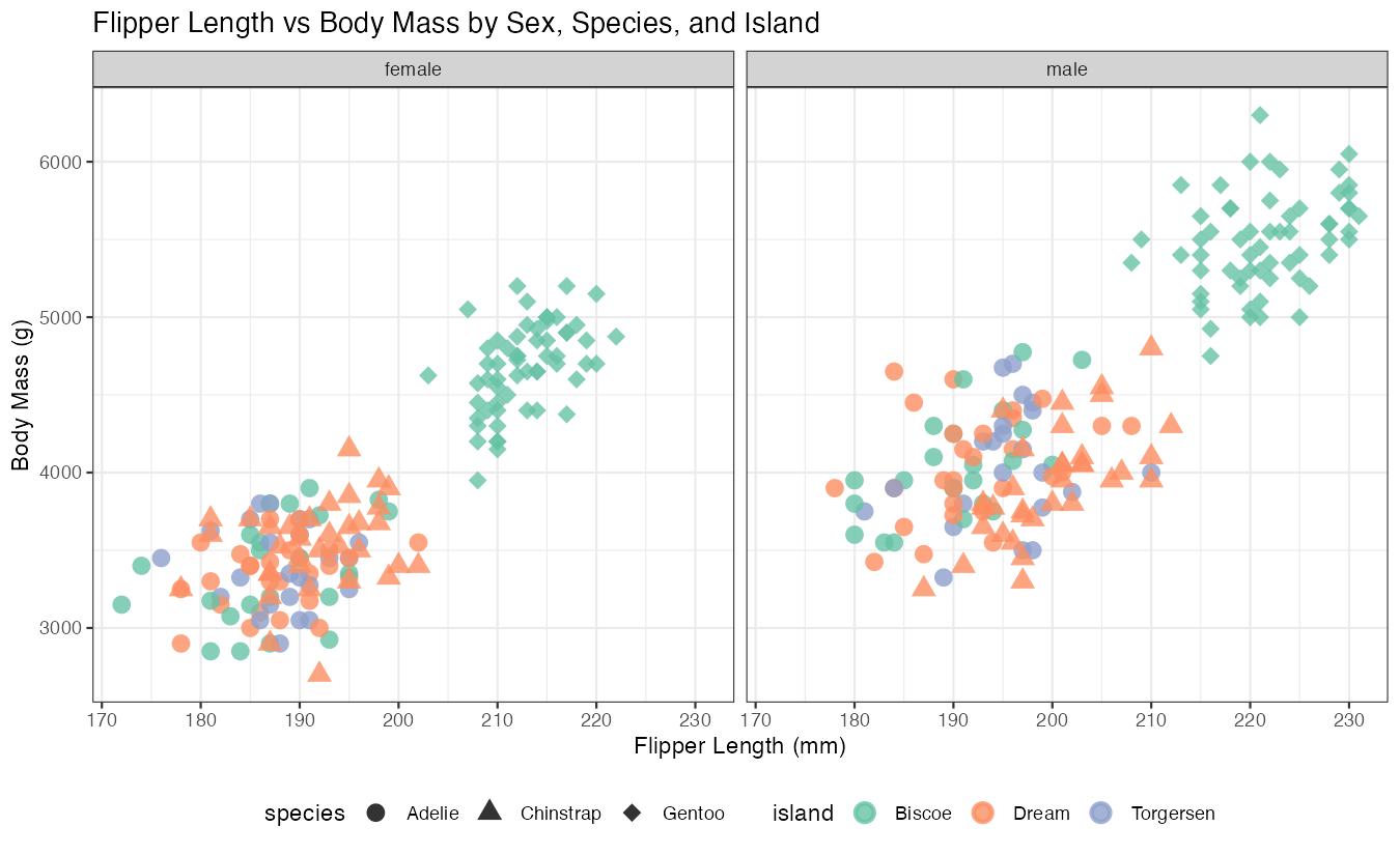
This advanced example showcases geom_point()’s full potential by combining shape mapping, faceting, and custom styling. The stroke parameter controls the outline width for certain point shapes, while custom shape values (16, 17, 18) provide distinct symbols for each species. Faceting by sex creates separate panels, making it easy to compare patterns across male and female penguins.
Common Mistakes
1. Overplotting without transparency:
# Problem: Points obscure each other
ggplot(penguins, aes(x = bill_length_mm, y = bill_depth_mm)) +
  geom_point(size = 5)

# Solution: Add transparency
ggplot(penguins, aes(x = bill_length_mm, y = bill_depth_mm)) +
  geom_point(size = 5, alpha = 0.6)
2. Ignoring missing values:
# Problem: Warning messages about removed rows
ggplot(penguins, aes(x = bill_length_mm, y = bill_depth_mm)) +
  geom_point()

# Solution: Handle NAs explicitly
ggplot(penguins, aes(x = bill_length_mm, y = bill_depth_mm)) +
  geom_point(na.rm = TRUE)
3. Mapping aesthetics incorrectly:
# Problem: Putting variable names in quotes
ggplot(penguins, aes(x = bill_length_mm, y = bill_depth_mm)) +
  geom_point(color = "species")  # Creates all blue points

# Solution: Use aes() for variable mapping
ggplot(penguins, aes(x = bill_length_mm, y = bill_depth_mm)) +
  geom_point(aes(color = species))  # Maps species to color