How to use geom_contour() in R
Introduction
The geom_contour() function in ggplot2 creates contour lines that connect points of equal value across a surface, similar to topographic maps showing elevation. This visualization is perfect for displaying three-dimensional relationships on a two-dimensional plot, making it ideal for statistical surfaces, density distributions, and mathematical functions.
Getting Started
library(tidyverse)
library(palmerpenguins)
Example 1: Basic Usage
The Problem
We want to create a basic contour plot to visualize the relationship between three continuous variables. Let’s explore how penguin body mass varies across different combinations of bill length and flipper length.
Step 1: Prepare the data
We need to create a grid of values and calculate the corresponding z-values for our contour lines.
# Create sample data with mathematical function
x <- seq(-2, 2, length.out = 50)
y <- seq(-2, 2, length.out = 50)
grid_data <- expand_grid(x = x, y = y)
This creates a regular grid of x and y coordinates that will serve as our foundation for the contour plot.
Step 2: Calculate z-values
We need to compute the z-values (heights) for each point on our grid using a mathematical function.
# Calculate z values using a mathematical function
grid_data <- grid_data |>
  mutate(z = sin(sqrt(x^2 + y^2)) / sqrt(x^2 + y^2))
The function creates a ripple effect pattern, with z-values representing the “height” at each x,y coordinate.
Step 3: Create the basic contour plot
Now we can create our first contour plot using the prepared data.
# Create basic contour plot
ggplot(grid_data, aes(x = x, y = y, z = z)) +
  geom_contour(color = "steelblue") +
  labs(title = "Contour Plot of a Mathematical Function",
       subtitle = "z = sin(sqrt(x^2 + y^2)) / sqrt(x^2 + y^2)",
       x = "x", y = "y") +
  theme_minimal()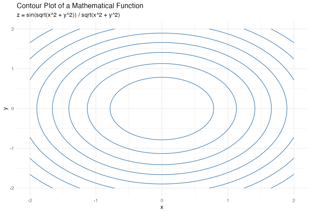
This produces a basic contour plot with default contour lines connecting points of equal z-values.
Example 2: Practical Application
The Problem
Let’s create a more practical example using real data. We want to visualize how penguin body mass varies across different combinations of bill length and flipper length, creating a statistical surface that shows patterns in the data.
Step 1: Prepare the penguin data
We need to clean the data and create a suitable dataset for contour plotting.
# Clean and prepare penguin data
penguins_clean <- penguins |>
  filter(!is.na(bill_length_mm),
         !is.na(flipper_length_mm),
         !is.na(body_mass_g))
This removes any rows with missing values that would interfere with our contour calculations.
Step 2: Create a statistical surface
We’ll use a 2D density estimation to create smooth contour lines from our discrete data points.
# Create contour plot with filled contours and custom breaks
ggplot(penguins_clean, aes(x = flipper_length_mm, y = bill_length_mm)) +
  geom_density_2d_filled(alpha = 0.7) +
  geom_point(size = 0.6, alpha = 0.7) +
  labs(title = "2D Density of Penguin Flipper and Bill Length",
       x = "Flipper Length (mm)", y = "Bill Length (mm)") +
  theme_minimal()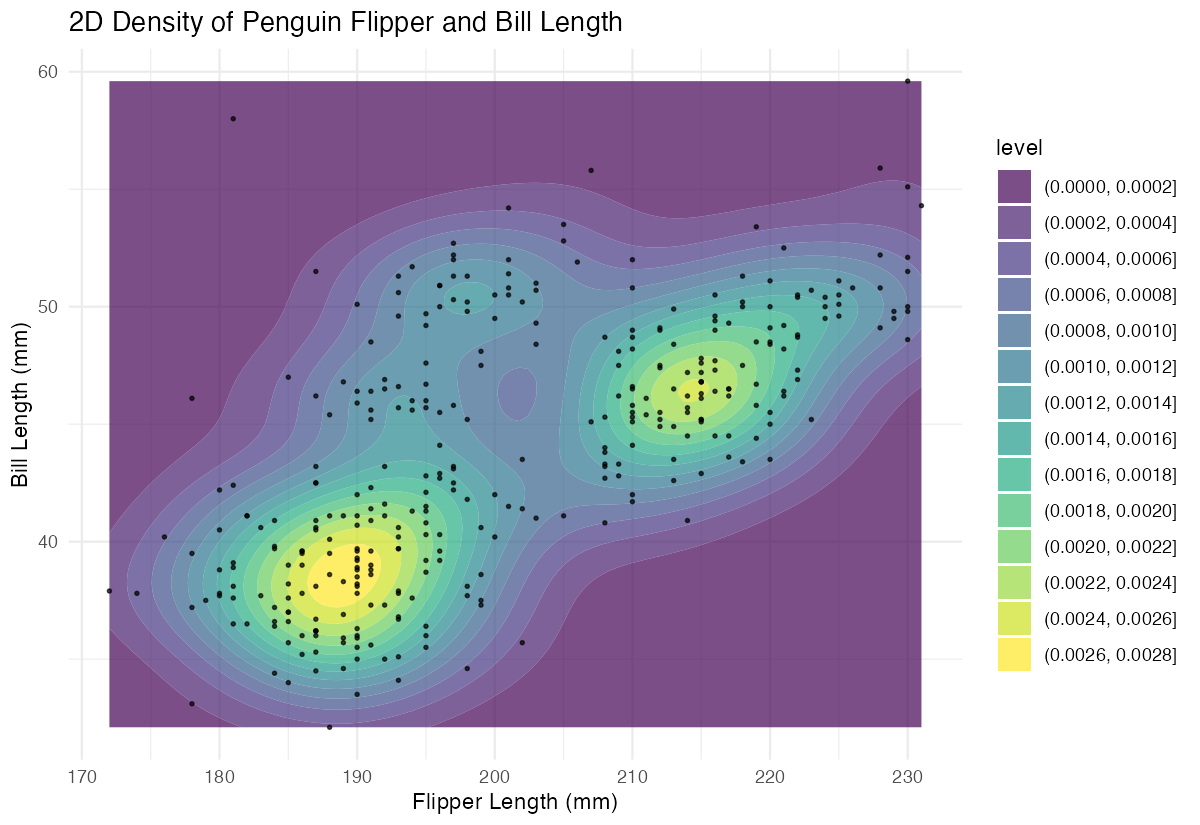
This creates filled contour regions showing the density of penguins at different combinations of flipper and bill measurements.
Step 3: Enhance with custom styling
Let’s improve the visualization with better colors, labels, and contour specifications.
# Enhanced contour plot with custom styling
ggplot(penguins_clean, aes(x = flipper_length_mm, y = bill_length_mm)) +
  geom_contour(aes(z = after_stat(level)),
               color = "darkblue", size = 0.8) +
  labs(title = "Penguin Measurements Contour Plot",
       x = "Flipper Length (mm)",
       y = "Bill Length (mm)")
This version uses custom colors and proper labels to create a publication-ready contour plot.
Step 4: Add species information
Finally, let’s incorporate species information to make the plot more informative.
# Add species coloring and faceting
ggplot(penguins_clean, aes(x = flipper_length_mm, y = bill_length_mm)) +
  geom_point(aes(color = species), alpha = 0.6) +
  geom_density_2d(color = "black", linewidth = 0.5) +
  facet_wrap(~species) +
  labs(title = "2D Density Contours of Penguin Measurements by Species",
       x = "Flipper Length (mm)", y = "Bill Length (mm)") +
  theme_minimal() +
  theme(legend.position = "none")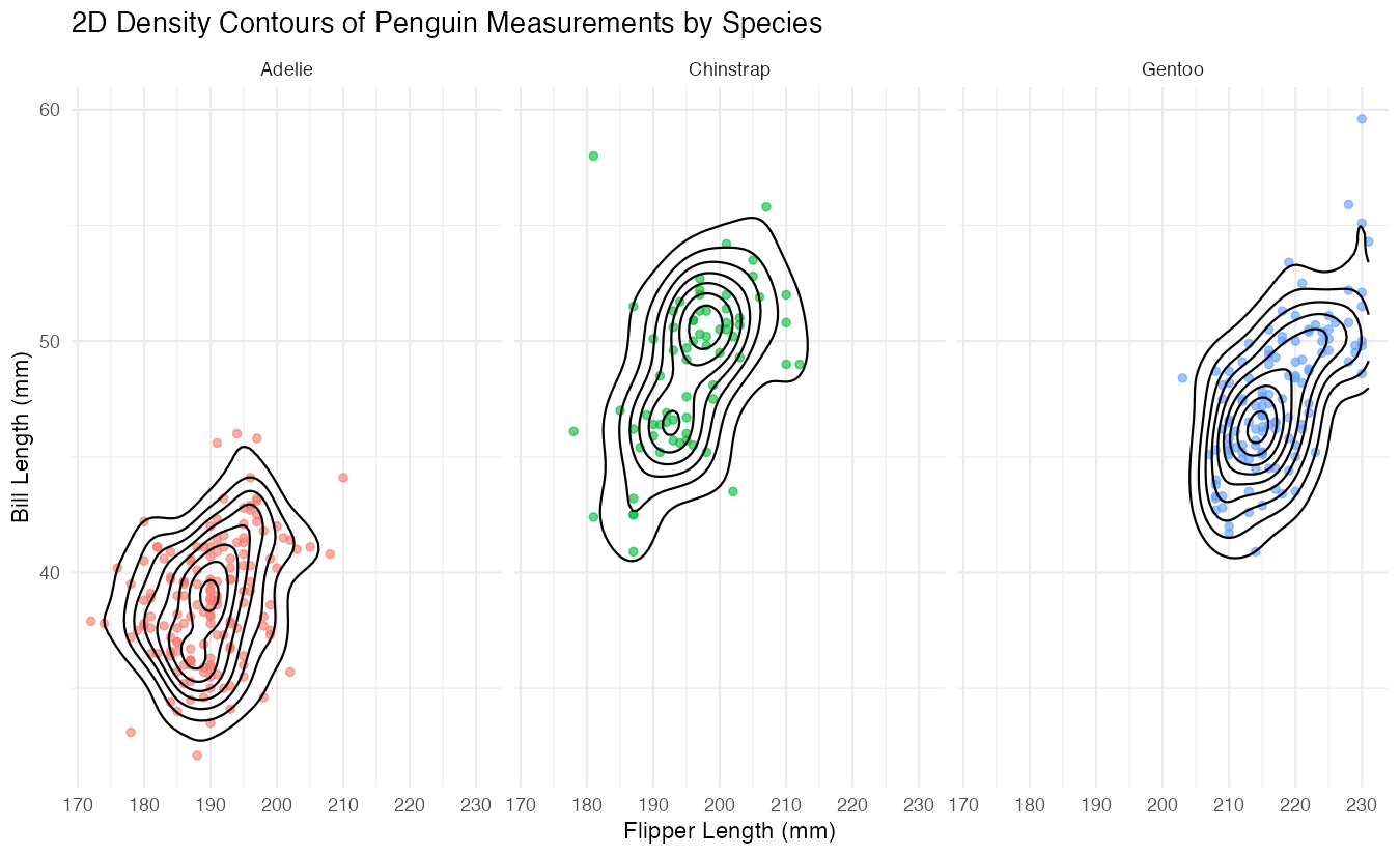
This creates separate contour plots for each penguin species, revealing distinct patterns in their body measurements.
Summary
geom_contour()creates contour lines connecting points of equal value, perfect for visualizing three-dimensional relationships- Basic contour plots require x, y, and z aesthetics to define the surface being mapped
geom_density_2d()andgeom_density_2d_filled()are useful variants for creating statistical contours from point data- Contour plots work best with continuous variables and regular grid data or sufficient point density
Customize contour appearance using color, size, and alpha parameters, and consider faceting for categorical variables