How to use geom_boxplot() in R
Introduction
The geom_boxplot() function in ggplot2 creates box-and-whisker plots that display the distribution of a continuous variable across different categories. Box plots are perfect for comparing distributions between groups and identifying outliers in your data.
Getting Started
library(tidyverse)
library(palmerpenguins)
Example 1: Basic Usage
The Problem
You want to visualize how penguin body mass varies across different species. A box plot will show you the median, quartiles, and potential outliers for each species.
Step 1: Create a Simple Box Plot
We’ll start with the most basic box plot using penguin data.
ggplot(penguins, aes(x = species, y = body_mass_g)) +
  geom_boxplot()
This creates a box plot showing body mass distribution for each penguin species, with the median line clearly visible in each box.
Step 2: Add Color to Distinguish Groups
Let’s make the plot more visually appealing by adding colors for each species.
ggplot(penguins, aes(x = species, y = body_mass_g, fill = species)) +
  geom_boxplot() +
  scale_fill_viridis_d()
Now each species has a distinct color, making it easier to distinguish between the three penguin species in our dataset.
Step 3: Customize the Appearance
We’ll add proper labels and remove the redundant legend since species are labeled on the x-axis.
ggplot(penguins, aes(x = species, y = body_mass_g, fill = species)) +
  geom_boxplot() +
  scale_fill_viridis_d() +
  labs(title = "Penguin Body Mass by Species",
       x = "Species", y = "Body Mass (g)") +
  theme(legend.position = "none")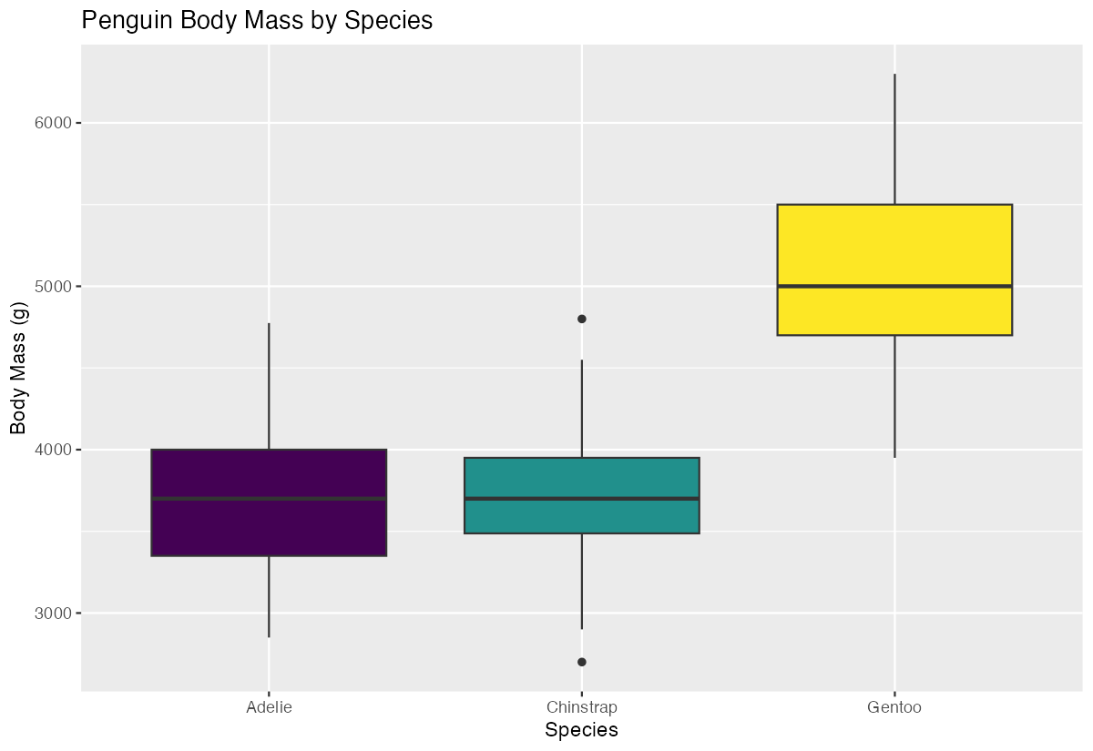
The plot now has clear labels and a clean appearance without the unnecessary legend.
Example 2: Practical Application
The Problem
You’re analyzing car performance data and want to compare fuel efficiency (mpg) across different numbers of cylinders. You also want to overlay individual data points to see the actual distribution and identify specific outliers.
Step 1: Prepare the Data
First, let’s convert cylinders to a factor for better grouping in our box plot.
mtcars_clean <- mtcars |>
  mutate(cyl_factor = factor(cyl)) |>
  select(mpg, cyl_factor, wt)
This creates a clean dataset with cylinders as a categorical variable, which works better with box plots.
Step 2: Create Box Plot with Data Points
We’ll create a box plot and overlay the actual data points using geom_jitter().
ggplot(mtcars_clean, aes(x = cyl_factor, y = mpg)) +
  geom_boxplot(alpha = 0.7, fill = "lightblue") +
  geom_jitter(width = 0.2, alpha = 0.6, color = "darkred")
The transparent box plots show the summary statistics while the jittered points reveal the actual data distribution and sample sizes.
Step 3: Add Statistical Notches
Let’s add notches to help compare medians between groups statistically.
ggplot(mtcars_clean, aes(x = cyl_factor, y = mpg, fill = cyl_factor)) +
  geom_boxplot(notch = TRUE, alpha = 0.8) +
  geom_jitter(width = 0.2, alpha = 0.6) +
  scale_fill_brewer(palette = "Set2")
Notches provide a visual test for comparing medians - if notches don’t overlap, the medians are significantly different.
Step 4: Final Polish
We’ll add professional labels and formatting for a publication-ready plot.
ggplot(mtcars_clean, aes(x = cyl_factor, y = mpg, fill = cyl_factor)) +
  geom_boxplot(notch = TRUE, alpha = 0.8) +
  geom_jitter(width = 0.2, alpha = 0.6) +
  scale_fill_brewer(palette = "Set2", name = "Cylinders") +
  labs(title = "Fuel Efficiency by Engine Configuration",
       subtitle = "Notches show 95% confidence interval around median",
       x = "Number of Cylinders", y = "Miles per Gallon") +
  theme_minimal()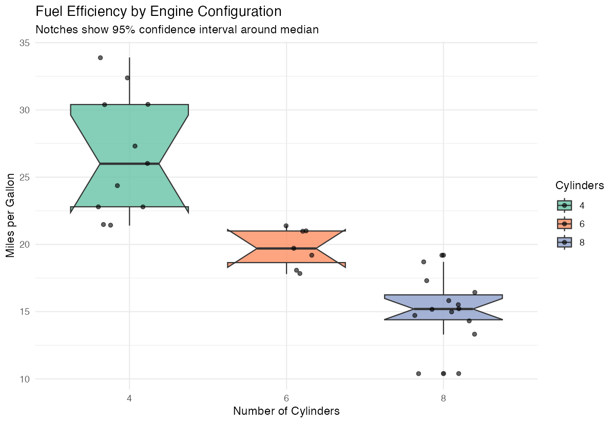
The final plot clearly shows that cars with fewer cylinders tend to have better fuel efficiency, with non-overlapping notches confirming significant differences.
Summary
- Use
geom_boxplot()to compare distributions across categorical groups - Add
fillaesthetic to distinguish groups with colors - Include
notch = TRUEto test for significant differences between medians
- Combine with
geom_jitter()to show individual data points alongside summaries Always add clear labels and consider removing redundant legends for cleaner presentation