How to use facet_wrap() in R
1. Introduction
The facet_wrap() function from the ggplot2 package creates multiple panels (subplots) of the same plot type, with each panel showing a subset of the data based on one or more categorical variables. This technique, known as “small multiples” or “panel plots,” allows you to easily compare patterns across different groups in your data.
You would use facet_wrap() when you want to visualize how relationships between variables differ across categories, compare distributions across groups, or reduce overplotting in dense datasets. It’s particularly useful for exploratory data analysis and when presenting complex multi-dimensional data in an easily digestible format. The function is part of the ggplot2 package, which is included in the tidyverse collection.
2. Syntax
facet_wrap(facets, nrow = NULL, ncol = NULL, scales = "fixed",
           shrink = TRUE, labeller = "label_value", as.table = TRUE,
           switch = NULL, drop = TRUE, dir = "h", strip.position = "top")
Key arguments: - facets: Formula or character vector specifying variables to facet by (e.g., ~species or vars(species)) - nrow, ncol: Number of rows and columns in the panel layout - scales: Whether scales should be “fixed” (default), “free”, “free_x”, or “free_y” - labeller: Function to customize panel labels - as.table: If TRUE, facets are laid out like a table with highest values at bottom-right - drop: If TRUE, drops unused factor levels
3. Example 1: Basic Usage
Let’s start with a simple example using the palmerpenguins dataset to create separate scatter plots for each penguin species:
library(tidyverse)
library(palmerpenguins)

# Basic facet_wrap usage
ggplot(penguins, aes(x = bill_length_mm, y = bill_depth_mm)) +
  geom_point(aes(color = sex)) +
  facet_wrap(~species) +
  labs(title = "Bill Length vs Depth by Species",
       x = "Bill Length (mm)",
       y = "Bill Depth (mm)")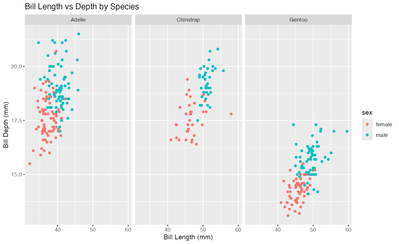
This creates three panels, one for each penguin species (Adelie, Chinstrap, Gentoo). Each panel shows the same scatter plot of bill length versus bill depth, colored by sex. The ~species formula tells facet_wrap() to create separate panels based on the unique values in the species column. By default, all panels share the same x and y axis scales, making it easy to compare the relationships across species.
4. Example 2: Practical Application
Here’s a more complex example analyzing penguin body mass distribution across species and islands, using free scales and custom layout:
# Remove rows with missing data and create a practical visualization
penguins |>
  drop_na() |>
  ggplot(aes(x = body_mass_g, fill = sex)) +
  geom_histogram(bins = 15, alpha = 0.7, position = "identity") +
  facet_wrap(~species + island,
             scales = "free_y",
             ncol = 3,
             labeller = label_both) +
  scale_fill_viridis_d(option = "plasma", begin = 0.3, end = 0.8) +
  theme_minimal() +
  theme(strip.text = element_text(size = 10, face = "bold")) +
  labs(title = "Penguin Body Mass Distribution",
       subtitle = "By Species and Island (Free Y-scales)",
       x = "Body Mass (g)",
       y = "Count",
       fill = "Sex")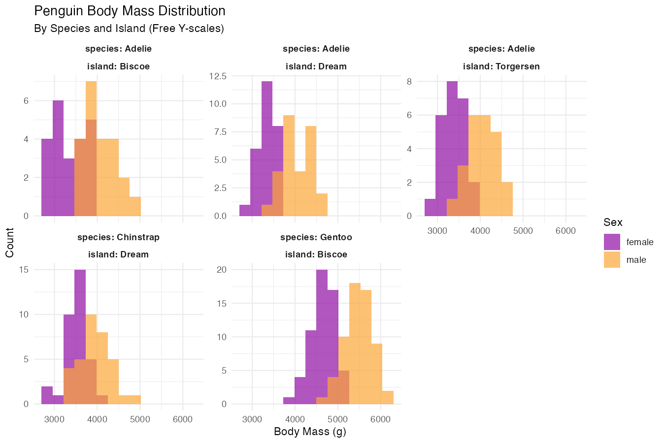
This example demonstrates several advanced features: combining multiple variables for faceting (species + island), using scales = "free_y" to allow different y-axis scales for each panel, controlling layout with ncol = 3, and using label_both to show both variable names and values in panel labels. The pipe syntax makes the data cleaning step seamless.
5. Example 3: Advanced Usage
Here’s an advanced example showing time-series-like data with custom labeling and layout control:
# Create a more complex visualization with year simulation
penguins |>
  drop_na() |>
  # Simulate different years for demonstration
  mutate(year = sample(2018:2021, nrow(drop_na(penguins)), replace = TRUE)) |>
  ggplot(aes(x = flipper_length_mm, y = body_mass_g)) +
  geom_point(aes(color = species), alpha = 0.6) +
  geom_smooth(method = "lm", se = FALSE, color = "black", linewidth = 0.5) +
  facet_wrap(vars(year, island),
             nrow = 2,
             scales = "free",
             labeller = labeller(year = function(x) paste("Year", x),
                               island = function(x) paste(x, "Island"))) +
  scale_color_brewer(type = "qual", palette = "Set1") +
  theme_bw() +
  theme(panel.grid.minor = element_blank(),
        strip.background = element_rect(fill = "lightblue")) +
  labs(title = "Flipper Length vs Body Mass Trends",
       subtitle = "By Year and Island with Individual Regression Lines")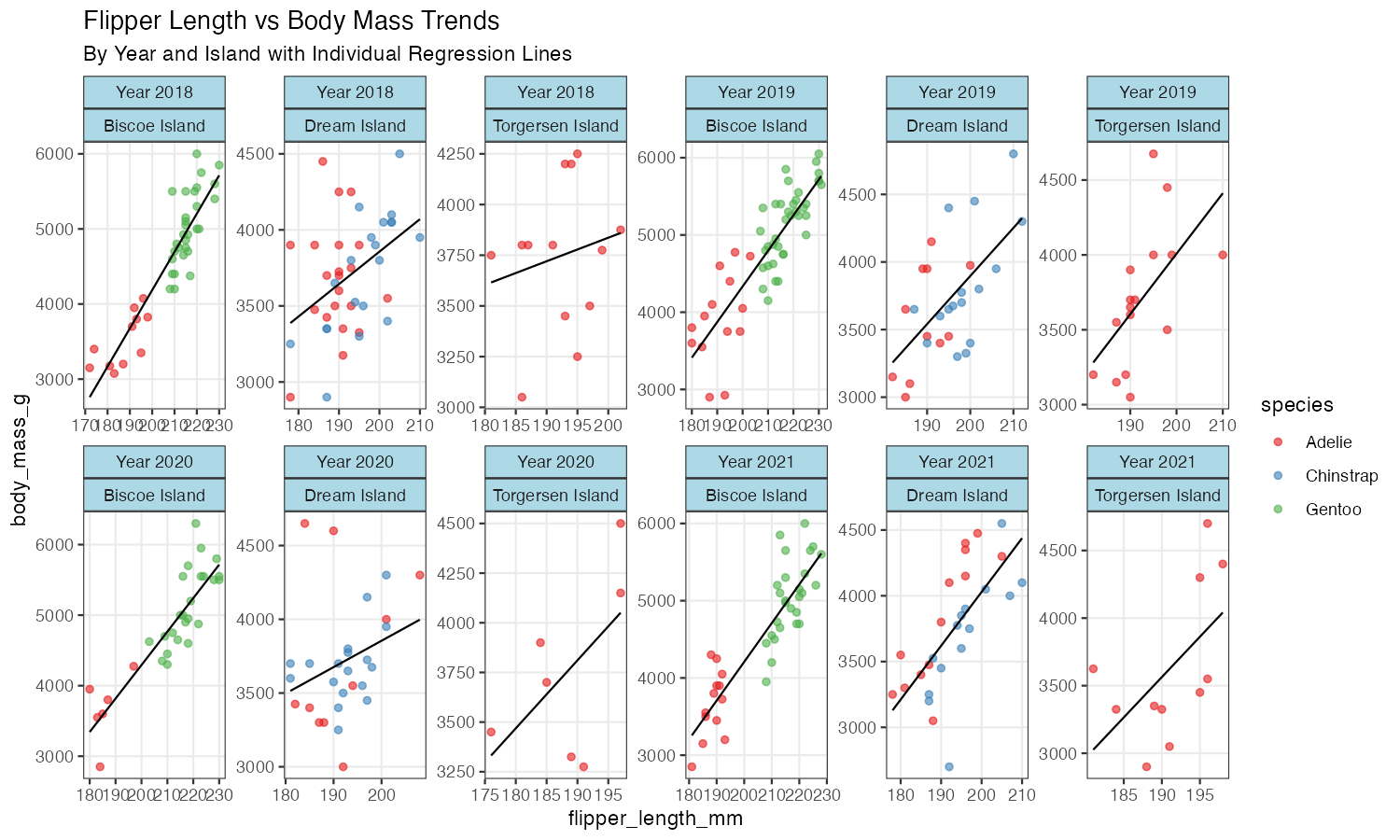
This advanced example uses vars() syntax for cleaner code, custom labeller functions, free scales on both axes, and combines multiple geoms with faceting for a comprehensive analysis view.
6. Common Mistakes
Mistake 1: Forgetting the tilde (~) in formula syntax
# Wrong
facet_wrap(species)

# Correct
facet_wrap(~species)
Mistake 2: Not handling missing values before faceting
# Can create unexpected empty panels or errors
ggplot(penguins, aes(x = bill_length_mm, y = bill_depth_mm)) +
  geom_point() +
  facet_wrap(~species)  # May show NA panel

# Better: filter or handle NAs first
penguins |> drop_na() |>
  ggplot(aes(x = bill_length_mm, y = bill_depth_mm)) +
  geom_point() +
  facet_wrap(~species)
Mistake 3: Using fixed scales when free scales would be more appropriate When the ranges differ dramatically between facets, fixed scales can make some panels hard to read. Consider using scales = "free", scales = "free_x", or scales = "free_y" for better visibility.