How to use geom_bar() in R
Introduction
The geom_bar() function in ggplot2 creates bar charts by counting the number of cases in each group. It’s one of the most commonly used geoms for visualizing categorical data distributions. Unlike geom_col() which plots pre-calculated heights, geom_bar() automatically counts observations and displays the frequencies as bar heights. This function is essential for exploratory data analysis when you need to understand the distribution of categorical variables or compare counts across different groups. You’ll use geom_bar() when analyzing survey responses, demographic data, species counts, or any scenario where you want to visualize how frequently different categories appear in your dataset.
Syntax
geom_bar(
  mapping = NULL,
  data = NULL,
  stat = "count",
  position = "stack",
  ...,
  width = NULL,
  na.rm = FALSE,
  orientation = NA,
  show.legend = NA,
  inherit.aes = TRUE
)
Key arguments: - mapping: Aesthetic mappings (typically aes(x = variable)) - stat: Statistical transformation, default is “count” - position: Position adjustment (“stack”, “dodge”, “fill”) - width: Bar width (0-1, where 1 means bars touch) - fill/color: Inside color and border color of bars - alpha: Transparency (0 = transparent, 1 = opaque)
Example 1: Basic Usage
library(tidyverse)
library(palmerpenguins)

# Basic bar chart showing penguin species counts
ggplot(penguins, aes(x = species)) +
  geom_bar() +
  labs(title = "Count of Penguin Species",
       x = "Species",
       y = "Count")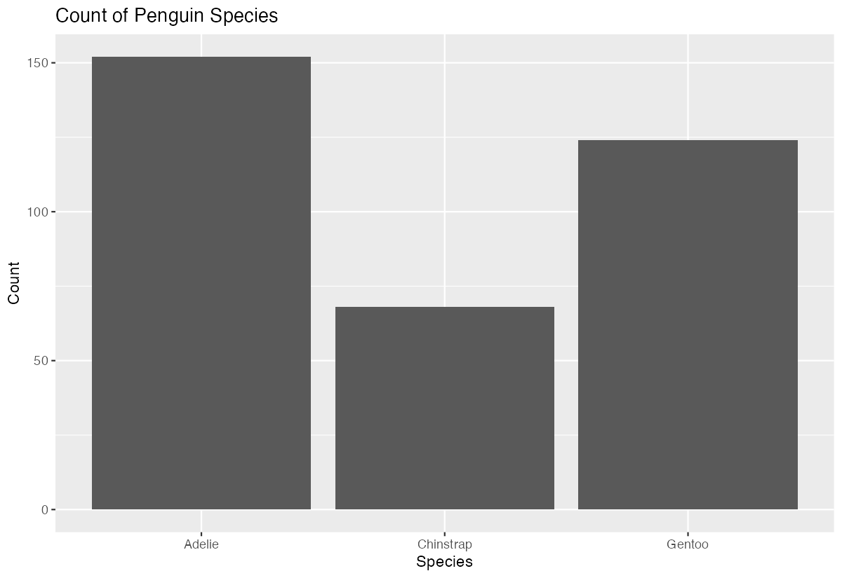
This creates a simple bar chart showing the frequency of each penguin species in the dataset. The bars automatically show that Adelie penguins are most common (152), followed by Gentoo (124), then Chinstrap (68). The geom_bar() function counted the observations for us - we didn’t need to calculate these frequencies beforehand.
Example 2: Practical Application
# Analyzing penguin species distribution by island with filled bars
penguins |>
  filter(!is.na(species), !is.na(island)) |>
  ggplot(aes(x = island, fill = species)) +
  geom_bar(position = "dodge", alpha = 0.8) +
  scale_fill_manual(values = c("darkorange", "purple", "cyan4")) +
  labs(title = "Penguin Species Distribution Across Islands",
       subtitle = "Each species has distinct island preferences",
       x = "Island",
       y = "Number of Penguins",
       fill = "Species") +
  theme_minimal() +
  theme(legend.position = "bottom")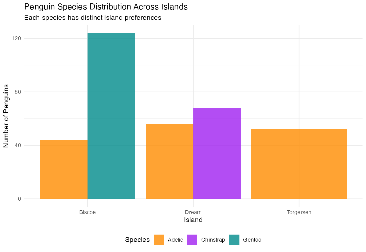
This practical example reveals important ecological patterns: Adelie penguins are found on all three islands, Chinstrap penguins only on Dream island, and Gentoo penguins exclusively on Biscoe island. The position = "dodge" places bars side-by-side for easy comparison, while the custom colors and clean theme make the visualization publication-ready.
Example 3: Advanced Usage
# Proportional stacked bars with custom styling
penguins |>
  filter(!is.na(species), !is.na(island), !is.na(sex)) |>
  ggplot(aes(x = island, fill = interaction(species, sex))) +
  geom_bar(position = "fill", width = 0.7) +
  scale_y_continuous(labels = scales::percent_format()) +
  scale_fill_brewer(type = "qual", palette = "Set3") +
  labs(title = "Species and Sex Composition by Island",
       x = "Island",
       y = "Proportion",
       fill = "Species.Sex") +
  theme_classic() +
  theme(axis.text.x = element_text(angle = 45, hjust = 1),
        legend.key.size = unit(0.8, "cm"))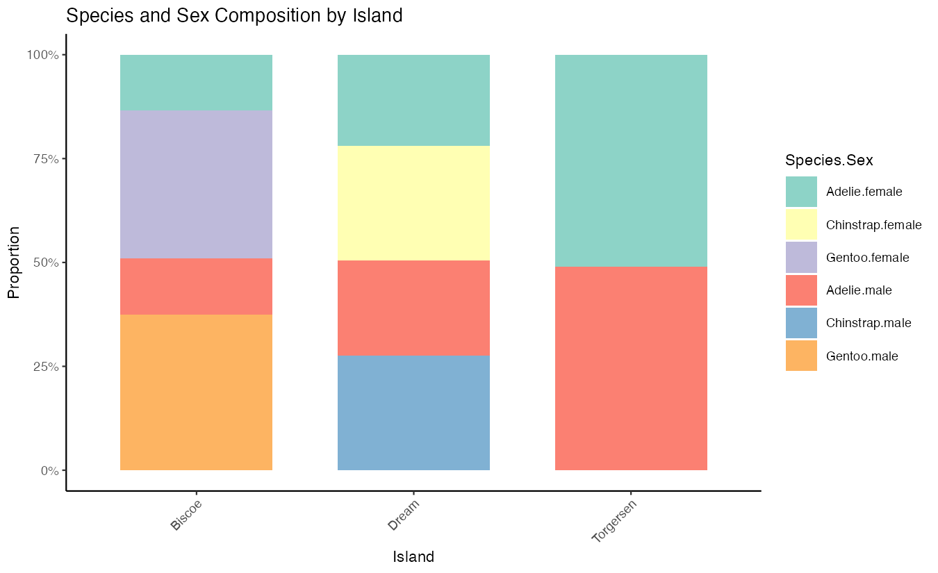
This advanced example uses position = "fill" to create proportional bars that sum to 100%, allowing comparison of relative compositions across islands. The interaction() function combines species and sex variables, while percentage formatting and custom width create a professional appearance. This reveals both species distribution and sex ratios within each island’s penguin population.
Common Mistakes
1. Confusing geom_bar() with geom_col()
# Wrong - trying to use pre-calculated values with geom_bar()
penguins |> count(species) |> ggplot(aes(x = species, y = n)) + geom_bar()

# Correct - use geom_col() for pre-calculated values
penguins |> count(species) |> ggplot(aes(x = species, y = n)) + geom_col()
2. Forgetting to handle missing values
# May produce warnings with NA values
ggplot(penguins, aes(x = sex)) + geom_bar()

# Better - filter out NAs first
penguins |> filter(!is.na(sex)) |> ggplot(aes(x = sex)) + geom_bar()
3. Using wrong position for grouped data
# Hard to read - bars are stacked by default
ggplot(penguins, aes(x = island, fill = species)) + geom_bar()

# Clearer - use position = "dodge" for side-by-side comparison
ggplot(penguins, aes(x = island, fill = species)) + geom_bar(position = "dodge")