How to use geom_col() in R
Introduction
The geom_col() function in ggplot2 creates column charts where the height of each bar represents values in your data. Unlike geom_bar() which counts observations, geom_col() uses the actual values from a specified column, making it perfect for displaying pre-calculated statistics, totals, or measurements.
Getting Started
library(tidyverse)
library(palmerpenguins)
Example 1: Basic Usage
The Problem
We want to create a simple column chart showing the average body mass of each penguin species. This requires calculating summary statistics and then visualizing them as columns.
Step 1: Calculate Summary Statistics
We need to group our data by species and calculate the mean body mass.
penguin_summary <- penguins |>
  filter(!is.na(body_mass_g)) |>
  group_by(species) |>
  summarise(avg_mass = mean(body_mass_g))

penguin_summary
This creates a summary table with species names and their corresponding average body masses.
Step 2: Create Basic Column Chart
Now we’ll use geom_col() to display these calculated values as columns.
ggplot(penguin_summary, aes(x = species, y = avg_mass)) +
  geom_col()
The function automatically creates bars with heights matching our avg_mass values for each species.
Step 3: Improve the Appearance
Let’s add better labels and formatting to make the chart more professional.
ggplot(penguin_summary, aes(x = species, y = avg_mass)) +
  geom_col(fill = "steelblue", alpha = 0.7) +
  labs(title = "Average Body Mass by Penguin Species",
       x = "Species",
       y = "Average Body Mass (g)")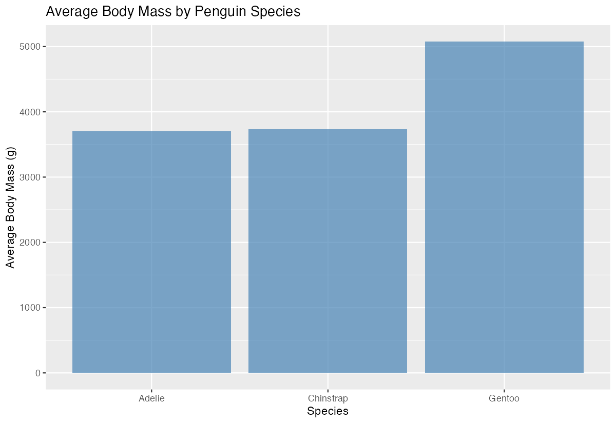
The chart now has color, transparency, and clear labels that make it publication-ready.
Example 2: Practical Application
The Problem
A researcher wants to compare total flipper length measurements across different islands, broken down by penguin species. This represents a real-world scenario where we need to show multiple categories and their relationships in a grouped column chart.
Step 1: Prepare Multi-Group Data
We’ll calculate total flipper lengths by both island and species to create grouped data.
flipper_data <- penguins |>
  filter(!is.na(flipper_length_mm)) |>
  group_by(island, species) |>
  summarise(total_flipper = sum(flipper_length_mm), .groups = "drop")

head(flipper_data)
This creates a dataset with totals for each combination of island and species.
Step 2: Create Grouped Column Chart
We’ll use the fill aesthetic to create side-by-side columns for each species.
ggplot(flipper_data, aes(x = island, y = total_flipper, fill = species)) +
  geom_col(position = "dodge")
The position = "dodge" argument places columns side-by-side rather than stacking them.
Step 3: Add Professional Styling
Let’s enhance the chart with custom colors and improved formatting.
ggplot(flipper_data, aes(x = island, y = total_flipper, fill = species)) +
  geom_col(position = "dodge", alpha = 0.8) +
  scale_fill_manual(values = c("Adelie" = "#FF6B6B",
                              "Chinstrap" = "#4ECDC4",
                              "Gentoo" = "#45B7D1"))
Custom colors make each species easily distinguishable and visually appealing.
Step 4: Finalize with Labels and Theme
Complete the visualization with comprehensive labels and a clean theme.
ggplot(flipper_data, aes(x = island, y = total_flipper, fill = species)) +
  geom_col(position = "dodge", alpha = 0.8) +
  scale_fill_manual(values = c("Adelie" = "#FF6B6B",
                              "Chinstrap" = "#4ECDC4",
                              "Gentoo" = "#45B7D1")) +
  labs(title = "Total Flipper Length by Island and Species",
       x = "Island", y = "Total Flipper Length (mm)",
       fill = "Species") +
  theme_minimal()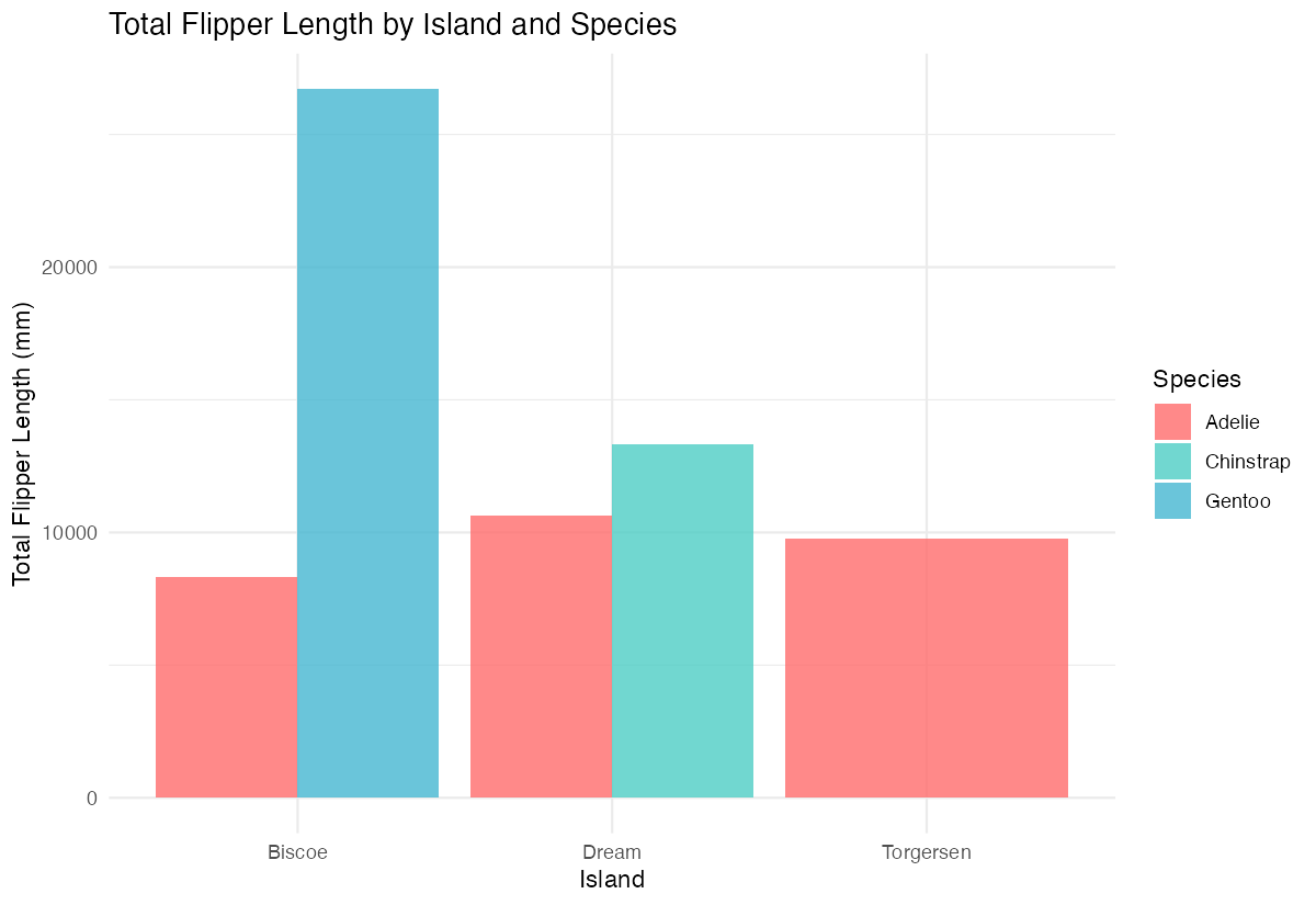
The final chart clearly shows the distribution and comparison of flipper measurements across all categories.
Summary
geom_col()uses actual data values to determine bar heights, unlikegeom_bar()which counts observations- Always prepare your data first by calculating the summary statistics you want to display
- Use
position = "dodge"to create side-by-side grouped columns instead of stacked bars - The
fillaesthetic creates multiple series within each x-axis category for comparative analysis Combine with custom colors, labels, and themes to create professional, publication-ready visualizations