How to use geom_histogram() in R
Introduction
The geom_histogram() function in ggplot2 creates histogram plots that show the distribution of a continuous variable by dividing data into bins and counting observations in each bin. Histograms are essential for exploring data distributions, identifying patterns like skewness or outliers, and understanding the shape of your data before conducting further analysis.
Getting Started
library(tidyverse)
library(palmerpenguins)
Example 1: Basic Usage
The Problem
We want to visualize the distribution of penguin body mass to understand how weights are spread across our dataset. This helps us identify the most common weight ranges and detect any unusual patterns.
Step 1: Create a Simple Histogram
We’ll start with the most basic histogram using default settings.
penguins |>
  ggplot(aes(x = body_mass_g)) +
  geom_histogram()
This creates a histogram with ggplot2’s default bin count (30 bins), showing the frequency distribution of penguin body mass.
Step 2: Customize Bin Width
Let’s control the bin width to get more meaningful groupings for our data.
penguins |>
  ggplot(aes(x = body_mass_g)) +
  geom_histogram(binwidth = 200) +
  labs(title = "Distribution of Penguin Body Mass",
       x = "Body Mass (g)")
Using a 200-gram bin width creates clearer groupings and reduces noise while maintaining the distribution’s overall shape.
Step 3: Improve Visual Appearance
Now we’ll add colors and borders to make the histogram more visually appealing.
penguins |>
  ggplot(aes(x = body_mass_g)) +
  geom_histogram(binwidth = 200,
                 fill = "skyblue",
                 color = "black",
                 alpha = 0.7)
The fill color, border, and transparency make the histogram more professional and easier to read.
Step 4: Add Statistical Information
Let’s include a vertical line showing the mean to add context to our distribution.
mean_mass <- mean(penguins$body_mass_g, na.rm = TRUE)

penguins |>
  ggplot(aes(x = body_mass_g)) +
  geom_histogram(binwidth = 200, fill = "skyblue", color = "black", alpha = 0.7) +
  geom_vline(xintercept = mean_mass, color = "red", linewidth = 1) +
  labs(title = "Distribution of Penguin Body Mass",
       subtitle = "Red line shows the mean",
       x = "Body Mass (g)", y = "Count")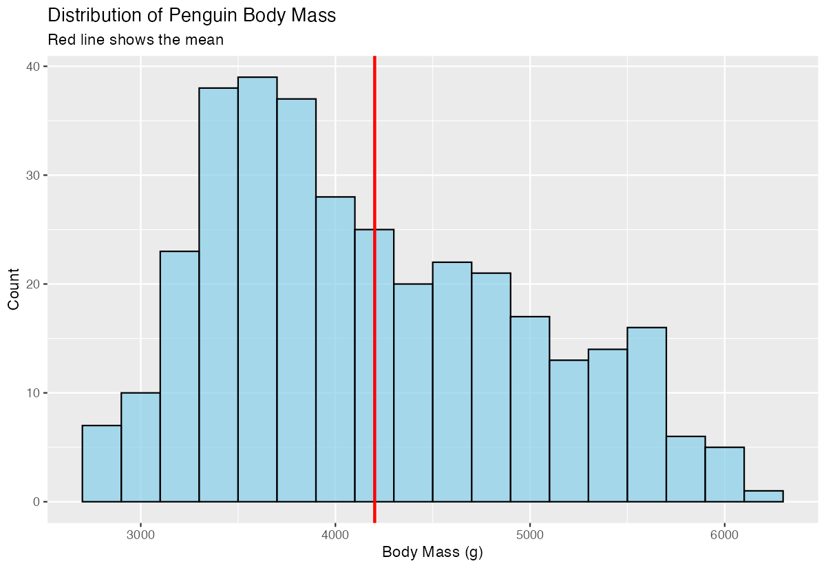
The red vertical line shows where the average body mass falls within the distribution, helping identify if the data is symmetric or skewed.
Example 2: Practical Application
The Problem
We need to compare body mass distributions across different penguin species to understand if there are distinct weight patterns. This comparison will help us identify which species tend to be larger or smaller and whether the distributions overlap significantly.
Step 1: Create Species-Specific Data
First, let’s filter out any missing values and examine our data structure.
clean_penguins <- penguins |>
  filter(!is.na(body_mass_g), !is.na(species))

clean_penguins |>
  count(species)
This ensures we have complete data for our analysis and shows us the sample size for each species.
Step 2: Create Faceted Histograms
We’ll create separate histograms for each species using faceting.
clean_penguins |>
  ggplot(aes(x = body_mass_g)) +
  geom_histogram(binwidth = 150, fill = "lightgreen", color = "black") +
  facet_wrap(~ species, ncol = 1) +
  labs(title = "Body Mass Distribution by Species")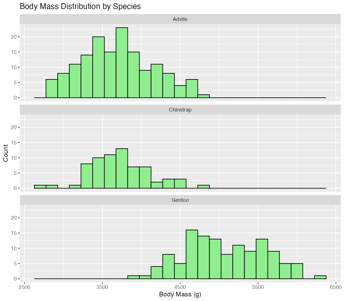
Faceting reveals that each species has a distinct distribution pattern, with Gentoo penguins showing notably higher body masses.
Step 3: Create Overlapping Histograms
Let’s overlay the distributions using different colors for direct comparison.
clean_penguins |>
  ggplot(aes(x = body_mass_g, fill = species)) +
  geom_histogram(binwidth = 150, alpha = 0.6, position = "identity") +
  scale_fill_manual(values = c("orange", "purple", "green")) +
  labs(title = "Overlapping Body Mass Distributions")
The overlapping histograms clearly show how Gentoo penguins are generally heavier, while Adelie and Chinstrap penguins have more similar, overlapping distributions.
Step 4: Calculate Summary Statistics
Finally, let’s add mean lines for each species to quantify the differences.
species_means <- clean_penguins |>
  group_by(species) |>
  summarise(mean_mass = mean(body_mass_g))

clean_penguins |>
  ggplot(aes(x = body_mass_g, fill = species)) +
  geom_histogram(binwidth = 150, alpha = 0.6, position = "identity") +
  geom_vline(data = species_means, aes(xintercept = mean_mass, color = species), linewidth = 1) +
  scale_fill_manual(values = c("orange", "purple", "green")) +
  scale_color_manual(values = c("orange", "purple", "green")) +
  labs(title = "Overlapping Body Mass Distributions by Species",
       x = "Body Mass (g)", y = "Count") +
  theme_minimal()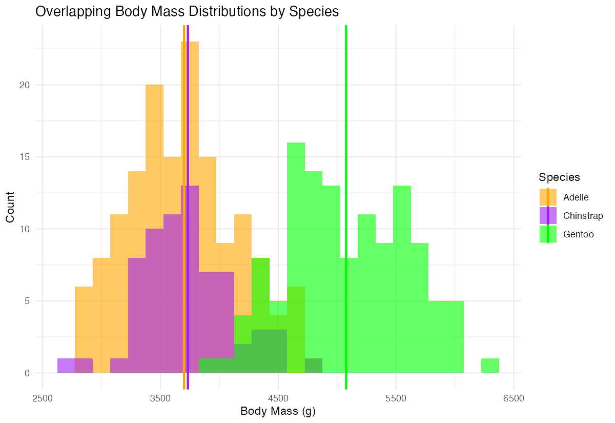
The colored vertical lines confirm our visual assessment, showing Gentoo penguins average about 1000g more than the other two species.
Summary
- Use
geom_histogram()to visualize the distribution of continuous variables and identify patterns in your data - Control bin width with the
binwidthparameter rather than relying on defaults for more meaningful visualizations - Enhance readability with fill colors, borders, and transparency using
fill,color, andalphaparameters - Compare groups effectively using either
facet_wrap()for separate panels or overlapping histograms with different colors Add context with statistical markers like mean lines using
geom_vline()to support visual interpretation