How to use facet_grid() in R
Introduction
The facet_grid() function in ggplot2 creates a grid of subplots based on the levels of one or more categorical variables. This powerful visualization tool allows you to compare patterns across different groups by arranging multiple plots in rows and columns. It’s particularly useful when you want to examine relationships while controlling for categorical variables.
Getting Started
library(tidyverse)
library(palmerpenguins)
Example 1: Basic Usage
The Problem
We want to explore the relationship between penguin bill length and depth, but we suspect this relationship might vary by species and sex. A single scatter plot would be cluttered and make it difficult to see patterns within each group.
Step 1: Create a Basic Scatter Plot
First, let’s create a simple scatter plot to see what we’re working with.
penguins |>
  ggplot(aes(x = bill_length_mm, y = bill_depth_mm)) +
  geom_point() +
  labs(title = "Penguin Bill Dimensions")
This shows all data points together, but it’s hard to distinguish patterns between different species or sexes.
Step 2: Add Single Variable Faceting
Now let’s split the data by species using facet_grid() with a single variable.
penguins |>
  ggplot(aes(x = bill_length_mm, y = bill_depth_mm)) +
  geom_point() +
  facet_grid(~ species) +
  labs(title = "Bill Dimensions by Species")
The ~ species syntax creates columns for each species, making it much easier to see distinct patterns within each group.
Step 3: Create a Two-Dimensional Grid
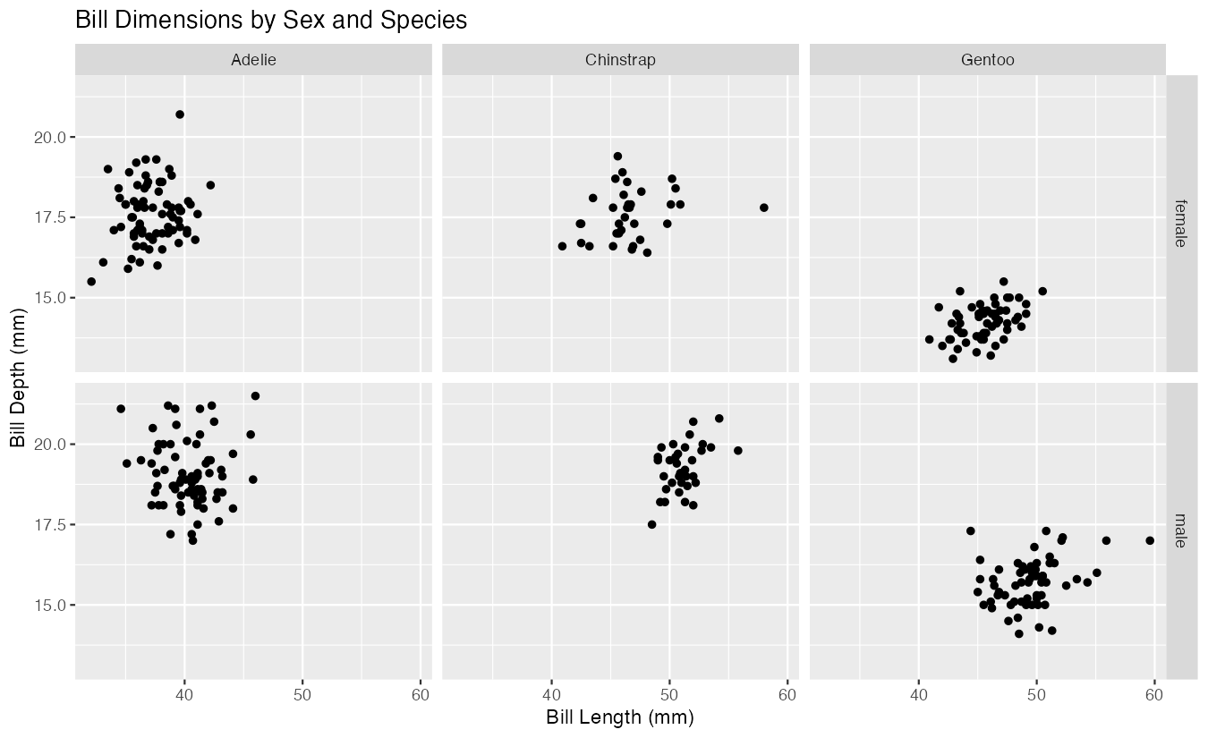
Let’s use both species and sex to create a more detailed grid.
penguins |>
  ggplot(aes(x = bill_length_mm, y = bill_depth_mm)) +
  geom_point() +
  facet_grid(sex ~ species) +
  labs(title = "Bill Dimensions by Sex and Species")
This creates a 2×3 grid where rows represent sex and columns represent species, allowing us to examine six different combinations simultaneously.
Example 2: Practical Application
The Problem
A researcher wants to analyze how car fuel efficiency (mpg) varies with engine power (horsepower) across different cylinder counts and transmission types. They need to present this complex relationship in a clear, organized manner that highlights patterns within each subgroup while maintaining comparability across groups.
Step 1: Prepare the Data
First, let’s prepare the mtcars dataset by converting relevant variables to factors.
mtcars_clean <- mtcars |>
  mutate(
    cyl = factor(cyl),
    am = factor(am, labels = c("Automatic", "Manual"))
  )
This converts cylinders and transmission type to factors with meaningful labels for better visualization.
Step 2: Create the Faceted Plot
Now let’s create a scatter plot with trend lines, faceted by our categorical variables.
mtcars_clean |>
  ggplot(aes(x = hp, y = mpg)) +
  geom_point(alpha = 0.7) +
  geom_smooth(method = "lm", se = FALSE) +
  facet_grid(am ~ cyl)
This creates a grid showing the horsepower-mpg relationship for each combination of transmission type and cylinder count, with trend lines for easy comparison.
Step 3: Enhance with Styling and Labels
Let’s improve the plot’s appearance and add informative labels.
mtcars_clean |>
  ggplot(aes(x = hp, y = mpg)) +
  geom_point(alpha = 0.7, color = "steelblue") +
  geom_smooth(method = "lm", se = FALSE, color = "red") +
  facet_grid(am ~ cyl, labeller = label_both) +
  labs(
    title = "Fuel Efficiency vs Engine Power",
    subtitle = "By transmission type and cylinder count",
    x = "Horsepower",
    y = "Miles per gallon"
  )
The labeller = label_both parameter adds variable names to the facet labels, making the plot more informative and professional.
![]()
Summary
facet_grid()creates subplot grids using the formula syntax:rows ~ columns- Use
~ variablefor single-dimension faceting (columns only) - Use
variable1 ~ variable2for two-dimensional grids - The
labellerparameter controls how facet labels appear Faceting works with any ggplot2 geometry and maintains consistent scales across subplots for easy comparison