How to Compute Z-Score of Multiple Columns
Introduction
Z-scores standardize data by measuring how many standard deviations a value is from the mean. Computing z-scores for multiple columns simultaneously is essential for data preprocessing, especially when preparing data for machine learning or comparing variables with different scales.
Getting Started
library(tidyverse)
library(palmerpenguins)
Example 1: Basic Z-Score Calculation
The Problem
We need to standardize multiple numeric columns in a dataset to make them comparable. Let’s start with the penguins dataset and standardize the body measurement columns.
Step 1: Prepare the Data
First, we’ll examine our dataset and select the numeric columns we want to standardize.
# Load and examine the penguins data
data(penguins)
head(penguins)

# Select numeric columns for z-score calculation
numeric_cols <- c("bill_length_mm", "bill_depth_mm",
                  "flipper_length_mm", "body_mass_g")
This gives us four body measurement columns that we’ll standardize.
Step 2: Calculate Z-Scores Using Base R
We’ll use the scale() function to compute z-scores for multiple columns at once.
# Calculate z-scores for selected columns
penguins_scaled <- penguins |>
  select(all_of(numeric_cols)) |>
  drop_na() |>
  scale() |>
  as_tibble()

head(penguins_scaled)
The scale() function automatically computes z-scores by subtracting the mean and dividing by the standard deviation for each column.
Step 3: Verify the Standardization
Let’s confirm our z-scores have mean ≈ 0 and standard deviation ≈ 1.
# Check means and standard deviations
penguins_scaled |>
  summarise(across(everything(),
                   list(mean = mean, sd = sd),
                   .names = "{.col}_{.fn}"))
Perfect! All means are essentially zero and standard deviations are 1, confirming our standardization worked correctly.
Example 2: Practical Application with Custom Function
The Problem
In real-world scenarios, you often need more control over the z-score calculation process. Let’s create a custom function that handles missing values better and allows us to keep other columns in our dataset.
Step 1: Create a Custom Z-Score Function
We’ll build a flexible function that can standardize selected columns while preserving the original dataset structure.
# Custom function to calculate z-scores
calculate_z_scores <- function(data, cols) {
  data |>
    mutate(across(all_of(cols),
                  ~ (. - mean(., na.rm = TRUE)) / sd(., na.rm = TRUE),
                  .names = "{.col}_z"))
}
This function creates new columns with “_z” suffix containing the standardized values.
Step 2: Apply the Function to Our Dataset
Now we’ll apply our custom function while keeping all original columns and handling missing values gracefully.
# Apply z-score calculation while keeping original data
penguins_with_z <- penguins |>
  calculate_z_scores(numeric_cols)

# View the results
penguins_with_z |>
  select(species, contains("_z")) |>
  head()
This approach preserves the original data while adding standardized versions, making it easier to compare different species’ measurements.
Step 3: Visualize the Standardized Data
Let’s create a visualization to see how standardization affects our data distribution.
# Compare original vs standardized distributions
penguins_with_z |>
  select(bill_length_mm, bill_length_mm_z) |>
  filter(!is.na(bill_length_mm)) |>
  pivot_longer(everything()) |>
  ggplot(aes(x = value, fill = name)) +
  geom_density(alpha = 0.7) +
  facet_wrap(~name, scales = "free") +
  labs(title = "Original vs Z-score Standardized Bill Length",
       x = "Value", y = "Density")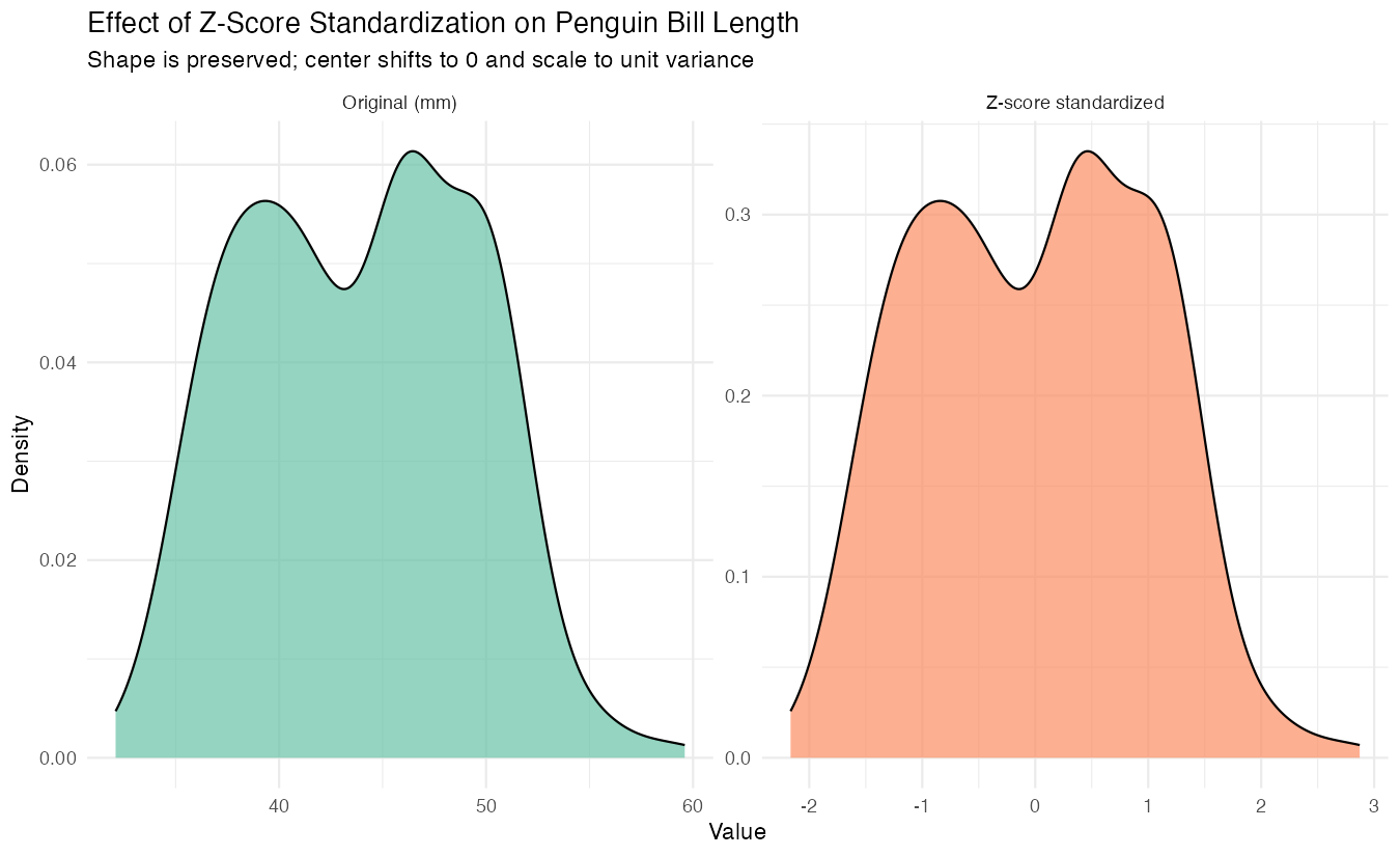
The standardized version shows the same distribution shape but centered at zero with unit variance.
Step 4: Compare Groups Using Z-Scores
Standardization makes it easy to compare measurements across different penguin species.
# Compare species using standardized measurements
penguins_with_z |>
  group_by(species) |>
  summarise(across(contains("_z"),
                   mean, na.rm = TRUE)) |>
  pivot_longer(-species,
               names_to = "measurement",
               values_to = "mean_z_score")
Now we can easily identify which species tend to be above or below average for each measurement.
Summary
- Z-scores standardize multiple columns by centering at mean 0 with standard deviation 1
- Use
scale()for quick standardization or create custom functions for more control - The
across()function withmutate()provides flexible column-wise operations - Standardization preserves distribution shape while making variables comparable
Z-scores are essential for machine learning preprocessing and comparative analysis