How to mean and median in R
Introduction
Mean and median are fundamental measures of central tendency that help you understand the typical value in your dataset. Use mean for normally distributed data and median when dealing with skewed data or outliers, as median is more resistant to extreme values.
Getting Started
library(tidyverse)
library(palmerpenguins)
Example 1: Basic Usage
The Problem
You need to calculate the average and middle value of a simple numeric vector. Let’s start with basic calculations using R’s built-in functions.
Step 1: Create sample data
We’ll create a vector of penguin body masses to work with.
# Extract body mass data
body_mass <- penguins$body_mass_g

# Remove missing values
body_mass_clean <- body_mass[!is.na(body_mass)]
This gives us a clean numeric vector without any missing values that could interfere with our calculations.
Step 2: Calculate the mean
The mean represents the arithmetic average of all values.
# Calculate mean body mass
mean_mass <- mean(body_mass_clean)
print(paste("Mean body mass:", round(mean_mass, 2), "grams"))
The mean tells us the average penguin weighs approximately 4,202 grams.
Step 3: Calculate the median
The median is the middle value when data is arranged in order.
# Calculate median body mass
median_mass <- median(body_mass_clean)
print(paste("Median body mass:", median_mass, "grams"))
The median shows that half of the penguins weigh less than 4,050 grams and half weigh more.
Step 4: Compare the results
Let’s see both values side by side to understand the data distribution.
# Compare mean and median
comparison <- data.frame(
  Statistic = c("Mean", "Median"),
  Value = c(mean_mass, median_mass)
)
print(comparison)
Since the mean is higher than the median, this suggests the data is slightly right-skewed with some heavier penguins.
Example 2: Practical Application
The Problem
You’re analyzing penguin data by species and need to calculate mean and median body mass for each group. This real-world scenario requires handling grouped data and missing values simultaneously.
Step 1: Group data by species
We’ll use the modern pipe operator to group our data efficiently.
# Group penguins by species
penguin_groups <- penguins |>
  filter(!is.na(body_mass_g)) |>
  group_by(species)
This creates grouped data where we can apply functions to each species separately.
Step 2: Calculate grouped statistics
Now we’ll compute both mean and median for each species in one operation.
# Calculate mean and median by species
species_stats <- penguin_groups |>
  summarise(
    mean_mass = mean(body_mass_g),
    median_mass = median(body_mass_g),
    .groups = 'drop'
  )
print(species_stats)
This shows clear differences between species, with Gentoo penguins being heaviest on average.
Step 3: Handle outliers with median
Let’s see how outliers affect our measures by comparing robust vs non-robust statistics.
# Add trimmed mean for comparison
species_comparison <- penguin_groups |>
  summarise(
    mean_mass = round(mean(body_mass_g), 1),
    median_mass = round(median(body_mass_g), 1),
    trimmed_mean = round(mean(body_mass_g, trim = 0.1), 1)
  )
The trimmed mean removes the top and bottom 10% of values, making it more similar to the median.
Step 4: Visualize the differences
A simple visualization helps us understand the distribution patterns.
# Create a summary plot — box center line is the median,
# red diamond marks the mean
species_stats <- penguins |>
  filter(!is.na(body_mass_g)) |>
  group_by(species) |>
  summarise(mean_mass = mean(body_mass_g), .groups = "drop")

penguins |>
  filter(!is.na(body_mass_g)) |>
  ggplot(aes(x = species, y = body_mass_g, fill = species)) +
  geom_boxplot(alpha = 0.7, outlier.shape = 1) +
  geom_point(data = species_stats,
             aes(x = species, y = mean_mass),
             shape = 23, fill = "red", color = "red", size = 4,
             inherit.aes = FALSE) +
  labs(title = "Penguin Body Mass by Species",
       subtitle = "Box center line shows the median; red diamond shows the mean",
       x = "Species", y = "Body Mass (g)") +
  theme_minimal() +
  theme(legend.position = "none")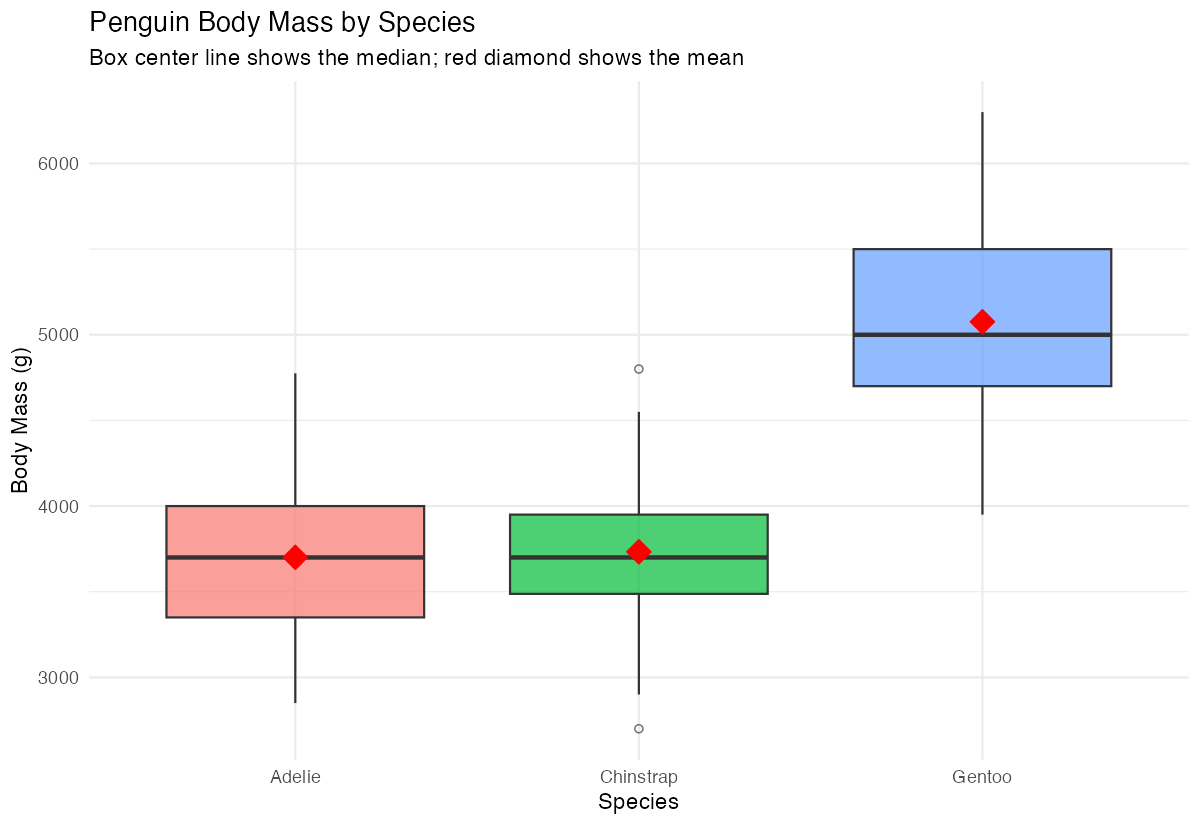
The boxplot clearly shows the median (center line) and helps identify which species have more outliers.
Summary
- Mean calculates the arithmetic average and works best with normally distributed data
- Median finds the middle value and is resistant to outliers and skewed distributions
- Use
mean()andmedian()functions, but always handle missing values first withna.rm = TRUEor filtering - Group calculations with
group_by()andsummarise()for analyzing categorical data Compare both statistics together to understand your data’s distribution and identify potential skewness