How to multiple linear regression in R
Introduction
Multiple linear regression is a statistical technique used to model the relationship between one continuous dependent variable and two or more independent variables. Unlike simple linear regression which uses only one predictor, multiple regression allows you to examine how several factors simultaneously influence your outcome variable.
This technique is particularly useful when you want to understand complex relationships in your data, make predictions based on multiple factors, or control for confounding variables. Common applications include predicting house prices based on size, location, and age, or analyzing how various factors affect student performance. Multiple regression helps quantify each variable’s unique contribution while accounting for the effects of other predictors in the model.
Getting Started
First, let’s load the necessary packages for our analysis:
library(tidyverse)
library(palmerpenguins)
Example 1: Basic Usage
Let’s start with a simple multiple regression using the mtcars dataset to predict fuel efficiency (mpg) based on weight (wt) and horsepower (hp):
data(mtcars)

model1 <- lm(mpg ~ wt + hp, data = mtcars)

summary(model1)
We can also examine the model’s performance and check assumptions:
par(mfrow = c(2, 2))
plot(model1)

anova(model1)
To make predictions with our model:
new_cars <- data.frame(wt = c(3.0, 3.5), hp = c(150, 200))
predict(model1, new_cars)
Example 2: Practical Application
Now let’s work with a more comprehensive example using the Palmer Penguins dataset. We’ll predict penguin body mass based on multiple morphological measurements:
penguins_clean <- penguins |>
  filter(!is.na(bill_length_mm),
         !is.na(bill_depth_mm),
         !is.na(flipper_length_mm),
         !is.na(body_mass_g)) |>
  select(body_mass_g, bill_length_mm, bill_depth_mm,
         flipper_length_mm, species, sex)

model2 <- penguins_clean |>
  lm(body_mass_g ~ bill_length_mm + bill_depth_mm + flipper_length_mm + species + sex,
     data = _)

summary(model2)
Let’s examine which variables contribute most to the model:
model_stats <- penguins_clean |>
  summarise(
    model = list(lm(body_mass_g ~ bill_length_mm + bill_depth_mm + flipper_length_mm + species + sex)),
    .groups = "drop"
  ) |>
  mutate(
    r_squared = map_dbl(model, ~ summary(.x)$r.squared),
    adj_r_squared = map_dbl(model, ~ summary(.x)$adj.r.squared)
  )

model_stats |>
  select(r_squared, adj_r_squared)
We can also create a more streamlined model by comparing different variable combinations:
models_comparison <- penguins_clean |>
summarise(
model_simple = list(lm(body_mass_g ~ flipper_length_mm, data = cur_data())),
model_full = list(lm(body_mass_g ~ bill_length_mm + bill_depth_mm + flipper_length_mm + species + sex, data = cur_data())),
.groups = "drop"
) |>
pivot_longer(cols = starts_with("model_"),
names_to = "model_type",
values_to = "model") |>
mutate(
aic = map_dbl(model, AIC),
r_squared = map_dbl(model, ~ summary(.x)$r.squared)
)
models_comparison |>
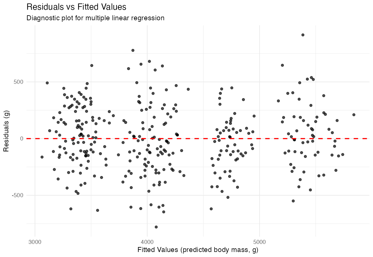
select(model_type, aic, r_squared)To visualize residuals and check model assumptions:
penguins_clean |>
  mutate(
    predicted = predict(model2),
    residuals = residuals(model2)
  ) |>
  ggplot(aes(x = predicted, y = residuals)) +
  geom_point(alpha = 0.7) +
  geom_hline(yintercept = 0, linetype = "dashed", color = "red", linewidth = 0.8) +
  labs(title = "Residuals vs Fitted Values",
       x = "Fitted Values",
       y = "Residuals") +
  theme_minimal()