# Load required packages
library(tidyverse)   # https://www.tidyverse.org/
library(scales)      # For nice axis formatting

# Set seed for reproducibility
set.seed(42)Introduction to Empirical Bayes in R
statistics
bayesian
empirical bayes
Learn Empirical Bayes estimation in R - a practical approach to improving estimates when you have many small samples. Includes product ratings example with step-by-step code.
Introduction
You’re shopping online and see two products:
- Product A: 5.0 stars from 3 reviews
- Product B: 4.2 stars from 500 reviews
Which one is actually better?
Your gut says Product B - and you’re right! A perfect 5-star rating from just 3 people could easily be luck (or fake reviews). But how do we formalize this intuition?
Empirical Bayes solves this problem elegantly. The key idea:
- Learn what’s typical - Most products have ratings between 3.5 and 4.5 stars
- Adjust extreme values - Pull suspiciously high (or low) ratings toward the average
- Adjust more for small samples - A 5-star rating from 3 reviews gets pulled down significantly; a 5-star rating from 500 reviews barely budges
This “shrinkage” reflects a simple truth: extreme results from small samples are usually luck, not skill. Empirical Bayes formalizes your gut instinct mathematically.
It’s a practical, powerful technique used in:
- Product rankings (Amazon, Yelp, App Store)
- Restaurant ratings
- A/B testing (which variant is really better?)
- Hospital/school rankings
- Any situation with many items, varying sample sizes
The Small Sample Problem
Let’s make this concrete with simulated product data.
Simulating Product Ratings
We’ll create 1,000 products with “true” quality levels, then simulate their actual reviews. Some products have many reviews, others have just a few.
# Simulate 1000 products
n_products <- 1000

# True product quality follows a Beta distribution
# Most products are decent (3-4 stars), few are terrible or amazing
# Beta(8, 2) gives mean ≈ 0.80 (translates to ~4 stars out of 5)
true_quality <- rbeta(n_products, shape1 = 8, shape2 = 2)

# Each product gets a random number of reviews
# Many products have few reviews, some have many
n_reviews <- sample(
  c(1:20, 25, 30, 50, 100, 200, 500, 1000),
  n_products,
  replace = TRUE,
  prob = c(rep(5, 20), 3, 3, 2, 2, 1, 1, 1)  # Most have few reviews
)

# Simulate positive reviews (5-star) based on true quality
positive_reviews <- rbinom(n_products, size = n_reviews, prob = true_quality)

# Create data frame
products <- tibble(
  product_id = 1:n_products,
  true_quality = true_quality,
  n_reviews = n_reviews,
  positive_reviews = positive_reviews,
  raw_rating = positive_reviews / n_reviews
)

head(products, 10)
# A tibble: 10 × 5
product_id true_quality n_reviews positive_reviews raw_rating
<int> <dbl> <dbl> <int> <dbl>
1 1 0.874 8 8 1
2 2 0.738 8 8 1
3 3 0.683 19 13 0.684
4 4 0.730 12 9 0.75
5 5 0.816 17 11 0.647
6 6 0.446 100 37 0.37
7 7 0.814 1 0 0
8 8 0.809 13 11 0.846
9 9 0.508 14 6 0.429
10 10 0.945 17 16 0.941Understanding the Data
| Variable | Description |
|---|---|
| true_quality | The product’s actual quality (unknown in real life) |
| n_reviews | Number of reviews (sample size) |
| positive_reviews | Number of 5-star reviews |
| raw_rating | positive_reviews / n_reviews (the naive estimate) |
NoteSimplification
We’re modeling ratings as “proportion of 5-star reviews” for simplicity. Real rating systems are more complex (1-5 stars), but the same principles apply. The Beta-Binomial model works perfectly for binary outcomes like “positive vs not positive.”
The Distribution of Reviews
ggplot(products, aes(x = n_reviews)) +
  geom_histogram(bins = 30, fill = "steelblue", color = "white") +
  scale_x_log10() +
  labs(
    title = "Distribution of Reviews per Product",
    subtitle = "Most products have few reviews - this is where the problem lies",
    x = "Number of Reviews (log scale)",
    y = "Count"
  ) +
  theme_minimal()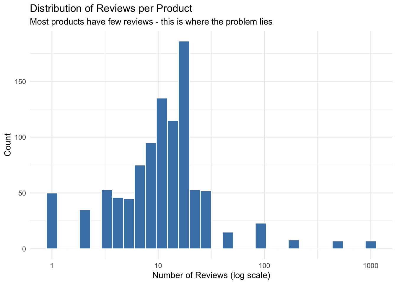
Visualizing the Problem
ggplot(products, aes(x = true_quality, y = raw_rating)) +
  geom_point(aes(size = n_reviews, color = n_reviews), alpha = 0.5) +
  geom_abline(slope = 1, intercept = 0, linetype = "dashed", color = "red") +
  scale_color_viridis_c(option = "plasma", trans = "log10") +
  scale_size_continuous(range = c(1, 8), trans = "log10") +
  labs(
    title = "Raw Ratings vs True Quality",
    subtitle = "Small samples (small dots) scatter wildly from the truth",
    x = "True Product Quality",
    y = "Raw Rating (Positive Reviews / Total)",
    size = "Reviews",
    color = "Reviews"
  ) +
  theme_minimal()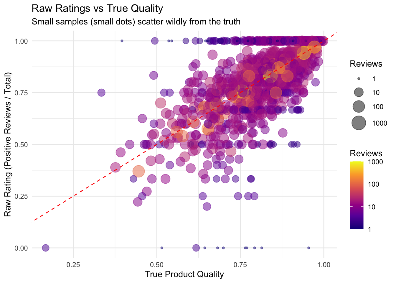
ImportantThe Problem is Clear
Products with few reviews (small dots) have ratings scattered far from their true quality. A product showing 100% positive from 3 reviews isn’t necessarily that good - they got lucky. Using raw ratings would mislead customers.
Quantifying the Error
# Compare error by sample size
products |>
  mutate(sample_size = case_when(
    n_reviews <= 5 ~ "Tiny (1-5)",
    n_reviews <= 20 ~ "Small (6-20)",
    n_reviews <= 100 ~ "Medium (21-100)",
    TRUE ~ "Large (100+)"
  ),
  sample_size = factor(sample_size, levels = c("Tiny (1-5)", "Small (6-20)",
                                                 "Medium (21-100)", "Large (100+)"))) |>
  group_by(sample_size) |>
  summarise(
    n_products = n(),
    mean_absolute_error = round(mean(abs(raw_rating - true_quality)), 3),
    .groups = "drop"
  )
# A tibble: 4 × 3
sample_size n_products mean_absolute_error
<fct> <int> <dbl>
1 Tiny (1-5) 229 0.202
2 Small (6-20) 659 0.086
3 Medium (21-100) 90 0.051
4 Large (100+) 22 0.012Products with tiny sample sizes have errors 5-10x larger than those with many reviews!
The Empirical Bayes Solution
The Key Insight
Instead of treating each product independently, we use information from all products to improve our estimate for each product.
The idea: 1. Estimate the overall distribution of product quality from the data 2. Combine each product’s raw rating with this prior knowledge 3. Shrink extreme ratings toward the population average
NoteWhy “Empirical” Bayes?
In traditional Bayesian statistics, you specify the prior distribution based on expert knowledge. In Empirical Bayes, you estimate the prior from the data itself - hence “empirical.”
Step 1: Estimate the Prior Distribution
We assume true product quality follows a Beta distribution. We estimate its parameters from the data using the method of moments.
# Method of moments estimation for Beta distribution
overall_mean <- sum(products$positive_reviews) / sum(products$n_reviews)
overall_var <- var(products$raw_rating)

# Estimate Beta parameters (alpha0, beta0)
alpha0 <- overall_mean * (overall_mean * (1 - overall_mean) / overall_var - 1)
beta0 <- (1 - overall_mean) * (overall_mean * (1 - overall_mean) / overall_var - 1)

cat("Estimated prior: Beta(", round(alpha0, 1), ", ", round(beta0, 1), ")\n")
Estimated prior: Beta( 2.6 , 0.6 )cat("Prior mean (average product quality):", round(alpha0 / (alpha0 + beta0), 3), "\n")Prior mean (average product quality): 0.814 This prior represents our belief about “typical” product quality before seeing any individual product’s reviews.
Step 2: Compute Posterior Estimates (Shrinkage!)
The magic of the Beta-Binomial model: the posterior estimate has a simple closed form.
# Empirical Bayes estimates
products <- products |>
  mutate(
    # Posterior estimate: weighted average of prior mean and raw rating
    eb_estimate = (positive_reviews + alpha0) / (n_reviews + alpha0 + beta0),

    # How much did we adjust?
    adjustment = eb_estimate - raw_rating
  )

products |>
  select(product_id, n_reviews, positive_reviews, raw_rating, eb_estimate, adjustment) |>
  head(10)
# A tibble: 10 × 6
product_id n_reviews positive_reviews raw_rating eb_estimate adjustment
<int> <dbl> <int> <dbl> <dbl> <dbl>
1 1 8 8 1 0.947 -0.0528
2 2 8 8 1 0.947 -0.0528
3 3 19 13 0.684 0.703 0.0186
4 4 12 9 0.75 0.763 0.0134
5 5 17 11 0.647 0.673 0.0263
6 6 100 37 0.37 0.384 0.0137
7 7 1 0 0 0.619 0.619
8 8 13 11 0.846 0.840 -0.00630
9 9 14 6 0.429 0.500 0.0713
10 10 17 16 0.941 0.921 -0.0200 The Shrinkage Formula
The Empirical Bayes estimate is:
\[\hat{p}_{EB} = \frac{\text{positive reviews} + \alpha_0}{\text{total reviews} + \alpha_0 + \beta_0}\]
This is a weighted average between: - The raw rating (positive / total) - The prior mean (α₀ / (α₀ + β₀))
More reviews → more weight on raw rating. Products with few reviews get pulled strongly toward the average.
# Show shrinkage with arrows for products with few reviews
set.seed(123)
sample_products <- products |>
  filter(n_reviews <= 20) |>
  sample_n(min(60, n()))

prior_mean <- alpha0 / (alpha0 + beta0)

ggplot(sample_products, aes(x = raw_rating, y = eb_estimate)) +
  geom_segment(aes(xend = raw_rating, yend = raw_rating),
               arrow = arrow(length = unit(0.15, "cm")), alpha = 0.4, color = "gray40") +
  geom_point(aes(color = n_reviews), size = 3) +
  geom_abline(slope = 1, intercept = 0, linetype = "dashed", color = "gray50") +
  geom_hline(yintercept = prior_mean, linetype = "dotted", color = "blue", linewidth = 1) +
  annotate("text", x = 0.35, y = prior_mean - 0.03,
           label = paste("Prior mean:", round(prior_mean, 2)), color = "blue", fontface = "bold") +
  scale_color_viridis_c(option = "plasma") +
  labs(
    title = "Shrinkage in Action",
    subtitle = "Arrows show movement from raw rating to Empirical Bayes estimate",
    x = "Raw Rating",
    y = "Empirical Bayes Estimate",
    color = "Reviews"
  ) +
  theme_minimal()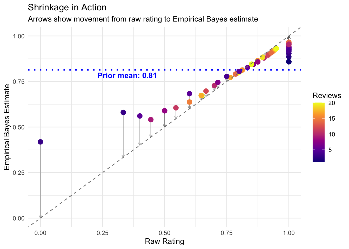
TipKey Insight
- Ratings far from the mean get pulled back (shrinkage)
- Products with few reviews shrink more
- Products with many reviews barely change (their data is trustworthy)
Step 3: Verify Improvement
Did shrinkage actually help? Let’s compare errors.
products |>
  mutate(
    error_raw = abs(raw_rating - true_quality),
    error_eb = abs(eb_estimate - true_quality),
    sample_size = case_when(
      n_reviews <= 5 ~ "Tiny\n(1-5)",
      n_reviews <= 20 ~ "Small\n(6-20)",
      n_reviews <= 100 ~ "Medium\n(21-100)",
      TRUE ~ "Large\n(100+)"
    ),
    sample_size = factor(sample_size, levels = c("Tiny\n(1-5)", "Small\n(6-20)",
                                                  "Medium\n(21-100)", "Large\n(100+)"))
  ) |>
  pivot_longer(cols = c(error_raw, error_eb),
               names_to = "method", values_to = "error") |>
  mutate(method = ifelse(method == "error_raw", "Raw Rating", "Empirical Bayes")) |>
  ggplot(aes(x = sample_size, y = error, fill = method)) +
  geom_boxplot() +
  scale_fill_manual(values = c("Raw Rating" = "#e74c3c", "Empirical Bayes" = "#27ae60")) +
  labs(
    title = "Empirical Bayes Dramatically Reduces Error",
    subtitle = "Biggest improvement for products with few reviews",
    x = "Number of Reviews",
    y = "Absolute Error from True Quality",
    fill = "Method"
  ) +
  theme_minimal()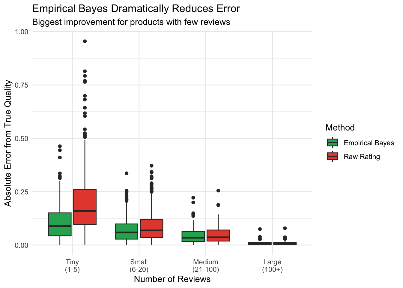
# Summary statistics
products |>
  summarise(
    mae_raw = mean(abs(raw_rating - true_quality)),
    mae_eb = mean(abs(eb_estimate - true_quality)),
    improvement_pct = round((mae_raw - mae_eb) / mae_raw * 100, 1)
  )
# A tibble: 1 × 3
mae_raw mae_eb improvement_pct
<dbl> <dbl> <dbl>
1 0.108 0.0752 30.4Empirical Bayes cuts the error substantially!
Credible Intervals
Beyond point estimates, we can quantify uncertainty using credible intervals from the posterior Beta distribution.
# Add credible intervals
products <- products |>
  mutate(
    # Posterior parameters for each product
    alpha_post = positive_reviews + alpha0,
    beta_post = (n_reviews - positive_reviews) + beta0,

    # 95% credible interval
    ci_low = qbeta(0.025, alpha_post, beta_post),
    ci_high = qbeta(0.975, alpha_post, beta_post),
    ci_width = ci_high - ci_low
  )

products |>
  select(product_id, n_reviews, raw_rating, eb_estimate, ci_low, ci_high, ci_width) |>
  arrange(n_reviews) |>
  head(10)
# A tibble: 10 × 7
product_id n_reviews raw_rating eb_estimate ci_low ci_high ci_width
<int> <dbl> <dbl> <dbl> <dbl> <dbl> <dbl>
1 7 1 0 0.619 0.179 0.956 0.777
2 13 1 0 0.619 0.179 0.956 0.777
3 42 1 1 0.859 0.445 1.00 0.554
4 67 1 1 0.859 0.445 1.00 0.554
5 127 1 1 0.859 0.445 1.00 0.554
6 149 1 1 0.859 0.445 1.00 0.554
7 163 1 1 0.859 0.445 1.00 0.554
8 175 1 1 0.859 0.445 1.00 0.554
9 199 1 1 0.859 0.445 1.00 0.554
10 217 1 1 0.859 0.445 1.00 0.554Notice how products with fewer reviews have wider intervals - we’re less certain about their true quality.
Visualizing Uncertainty
# Sample 30 products across range of review counts
set.seed(456)
sample_for_ci <- products |>
  arrange(n_reviews) |>
  mutate(row_num = row_number()) |>
  filter(row_num %in% round(seq(1, n(), length.out = 30)))

ggplot(sample_for_ci, aes(x = reorder(factor(product_id), n_reviews), y = eb_estimate)) +
  geom_errorbar(aes(ymin = ci_low, ymax = ci_high, color = n_reviews), width = 0.3) +
  geom_point(aes(color = n_reviews), size = 3) +
  geom_point(aes(y = true_quality), shape = 4, size = 2, color = "red") +
  scale_color_viridis_c(option = "plasma", trans = "log10") +
  labs(
    title = "Empirical Bayes Estimates with 95% Credible Intervals",
    subtitle = "Red X = true quality | More reviews = narrower intervals",
    x = "Product (ordered by number of reviews →)",
    y = "Quality Rating",
    color = "Reviews"
  ) +
  theme_minimal() +
  theme(axis.text.x = element_blank(), axis.ticks.x = element_blank())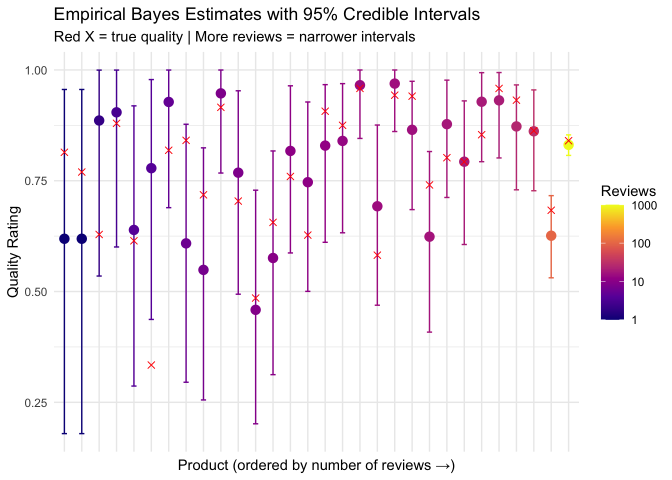
NoteInterpreting Credible Intervals
A 95% credible interval means: “Given our model, there’s a 95% probability the true quality lies in this range.” This is more intuitive than frequentist confidence intervals!
Ranking Products Fairly
Now we can rank products more fairly. Raw ratings favor products that got lucky with few reviews.
# Compare rankings
ranking_comparison <- products |>
  mutate(
    rank_raw = rank(-raw_rating),
    rank_eb = rank(-eb_estimate),
    rank_true = rank(-true_quality)
  )

# Top 10 by raw rating - are these really the best?
cat("Top 10 by Raw Rating:\n")
Top 10 by Raw Rating:ranking_comparison |>
arrange(rank_raw) |>
head(10) |>
select(product_id, n_reviews, raw_rating, eb_estimate, rank_raw, rank_true) |>
mutate(across(c(raw_rating, eb_estimate), ~round(., 3)))# A tibble: 10 × 6
product_id n_reviews raw_rating eb_estimate rank_raw rank_true
<int> <dbl> <dbl> <dbl> <dbl> <dbl>
1 1 8 1 0.947 124. 324
2 2 8 1 0.947 124. 742
3 14 5 1 0.928 124. 435
4 15 15 1 0.968 124. 8
5 20 25 1 0.979 124. 40
6 26 3 1 0.904 124. 791
7 27 6 1 0.936 124. 45
8 28 5 1 0.928 124. 246
9 29 2 1 0.886 124. 222
10 30 13 1 0.964 124. 9# Top 10 by Empirical Bayes
cat("Top 10 by Empirical Bayes:\n")Top 10 by Empirical Bayes:ranking_comparison |>
arrange(rank_eb) |>
head(10) |>
select(product_id, n_reviews, raw_rating, eb_estimate, rank_eb, rank_true) |>
mutate(across(c(raw_rating, eb_estimate), ~round(., 3)))# A tibble: 10 × 6
product_id n_reviews raw_rating eb_estimate rank_eb rank_true
<int> <dbl> <dbl> <dbl> <dbl> <dbl>
1 20 25 1 0.979 1.5 40
2 241 25 1 0.979 1.5 111
3 87 20 1 0.975 3.5 183
4 176 20 1 0.975 3.5 136
5 48 19 1 0.973 7 2
6 223 19 1 0.973 7 257
7 414 19 1 0.973 7 31
8 563 19 1 0.973 7 150
9 604 19 1 0.973 7 14
10 811 500 0.974 0.973 10 35The Empirical Bayes ranking identifies products that are actually good, not just lucky with small samples!
Real-World Applications
Where Empirical Bayes Shines
| Application | What’s Being Estimated | Why EB Helps |
|---|---|---|
| Amazon/Yelp Rankings | Product/restaurant quality | Many items have few reviews |
| App Store Ratings | App quality | New apps have limited data |
| A/B Testing | Conversion rates | Many tests with low traffic |
| Hospital Rankings | Quality of care | Small hospitals have extreme rates |
| School Ratings | Educational quality | Small schools are noisy |
| Sports Analytics | Player ability | Rookies have limited stats |
| Gene Expression | Expression levels | Thousands of genes, few samples |
TipWhen to Use Empirical Bayes
You have many similar units (products, hospitals, genes) with varying sample sizes, and you want to estimate something for each unit. The more units and the more variation in sample sizes, the more EB helps.
Quick Reference: The Procedure
Summary
- Raw ratings are misleading for products with few reviews
- Empirical Bayes shrinks extreme estimates toward a data-driven average
- More shrinkage for fewer reviews - small samples are less trustworthy
- Less shrinkage for many reviews - large samples speak for themselves
- Credible intervals honestly represent uncertainty
- Use when you have many units with varying sample sizes
Think of it this way: a 5-star rating from 3 reviews becomes ~4.5 stars after shrinkage, while a 5-star rating from 500 reviews stays at ~5.0 stars. That matches our intuition perfectly!
Frequently Asked Questions
Q: Why not just require a minimum number of reviews?
That’s a common approach (e.g., “must have 10+ reviews to be ranked”), but it wastes information. A product with 8 reviews still tells us something! Empirical Bayes uses all available data while appropriately discounting small samples.
Q: Is Empirical Bayes “cheating” by using the data twice?
You use data once to estimate the prior, then again to compute posteriors. In practice, when you have many units (100+), this “double-dipping” has minimal impact. For small numbers of units, consider full Bayesian methods.
Q: When should I use Empirical Bayes vs full Bayesian analysis?
Empirical Bayes is simpler and faster - great when you have many similar units and want quick, reasonable estimates. Full Bayesian analysis (with MCMC via Stan or brms) is better when you need full uncertainty propagation or have complex hierarchical structures.
Q: How many products/units do I need?
Rule of thumb: at least 20-30 units to estimate the prior reliably. With fewer units, consider using an informative prior based on domain knowledge instead.
Q: Can I use this for star ratings (1-5) instead of binary?
Yes! Options include: - Convert to binary (e.g., 4-5 stars = positive) - simplest - Use ordinal models - Model the mean rating with a Normal-Normal Empirical Bayes
Q: What about fake reviews?
Empirical Bayes doesn’t directly detect fakes, but it does reduce their impact. A product with 5 fake 5-star reviews will still be shrunk toward the mean. Combine with anomaly detection for best results.
Further Reading
- Introduction to Empirical Bayes - David Robinson’s classic blog series (uses baseball, but concepts apply)
- ebbr package - Tidyverse-friendly Empirical Bayes for R
- How Not To Sort By Average Rating - Evan Miller’s influential post on rating systems
- Empirical Bayes Methods in Statistics - Bradley Efron’s foundational paper