Introduction to Survival Analysis in R

Learn survival analysis in R with step-by-step examples. Covers Kaplan-Meier curves, log-rank tests, and Cox regression using real lung cancer data.

Introduction

A patient is diagnosed with advanced lung cancer and asks their doctor: “How long do I have?”

This question - estimating time until an event occurs - is at the heart of survival analysis. Despite its name, survival analysis isn’t just about death. It’s about modeling time-to-event data:

• Time until a patient dies (or recovers)
• Time until a customer cancels their subscription (churn)
• Time until a machine breaks down
• Time until a user makes their first purchase

The Censoring Problem

Here’s why we need special methods. Imagine following 5 patients for 2 years:

Patient	Month	Outcome	Status
A	8	Died	Observed
B	14	Died	Observed
C	24	Still alive (study ended)	Censored
D	10	Lost to follow-up (moved away)	Censored
E	20	Died	Observed

For Patients C and D, we know they survived at least that long, but we don’t know when (or if) they died. This is called right censoring - the most common type.

ImportantWhy Regular Methods Fail

If we just calculate average survival time, what do we do with Patient C (still alive at 24 months)? Ignoring them biases results downward. Treating 24 as their death time is also wrong. Survival analysis handles this correctly.

What You’ll Learn

In this tutorial, you’ll learn to:

1. Create and interpret Kaplan-Meier survival curves
2. Compare survival between groups using the log-rank test
3. Model survival with Cox proportional hazards regression
4. Interpret hazard ratios
5. Check model assumptions

Let’s dive in!

Setup

We’ll use three packages for survival analysis in R.

The survival package is R’s core survival analysis toolkit - it comes with R and provides all the fundamental functions.

library(survival)

The survminer package creates publication-quality survival plots using ggplot2.

library(survminer)

The tidyverse gives us data manipulation tools we’ll use throughout.

library(tidyverse)

The Dataset: Lung Cancer Survival

We’ll use the lung dataset from the survival package. It contains survival data from 228 patients with advanced lung cancer.

Let’s load and examine the data.

data(lung)
head(lung)

  inst time status age sex ph.ecog ph.karno pat.karno meal.cal wt.loss
1    3  306      2  74   1       1       90       100     1175      NA
2    3  455      2  68   1       0       90        90     1225      15
3    3 1010      1  56   1       0       90        90       NA      15
4    5  210      2  57   1       1       90        60     1150      11
5    1  883      2  60   1       0      100        90       NA       0
6   12 1022      1  74   1       1       50        80      513       0

Here’s what each variable means:

Variable	Description
time	Survival time in days
status	Censoring status: 1 = censored, 2 = dead
age	Age in years
sex	1 = Male, 2 = Female
ph.ecog	ECOG performance score (0 = good, 4 = bedridden)
ph.karno	Karnofsky performance score (physician rated)
pat.karno	Karnofsky score (patient rated)
meal.cal	Calories consumed at meals
wt.loss	Weight loss in last 6 months

The ECOG score is particularly important - it measures how well a patient can perform daily activities. A score of 0 means fully active; 4 means completely bedridden.

Data Preparation

First, let’s check the dimensions of our dataset.

dim(lung)

[1] 228  10

We have 228 patients and 10 variables.

Let’s recode sex to be more readable, and convert ph.ecog to a factor.

lung <- lung |>
  mutate(
    sex = factor(sex, levels = c(1, 2), labels = c("Male", "Female")),
    ph.ecog = factor(ph.ecog)
  )

Let’s see how many patients experienced the event (death) versus were censored.

lung |>
  count(status) |>
  mutate(status = ifelse(status == 1, "Censored", "Died"))

    status   n
1 Censored  63
2     Died 165

About 28% of patients were censored (still alive or lost to follow-up), and 72% died during the study.

Let’s also look at survival time distribution.

summary(lung$time)

   Min. 1st Qu.  Median    Mean 3rd Qu.    Max. 
    5.0   166.8   255.5   305.2   396.5  1022.0 

Survival times range from 5 to 1022 days (about 3 years), with a median of 226 days.

Creating Survival Objects

In R, survival data is stored in a special Surv object that pairs the time with the censoring status.

The Surv() function creates this object. It takes two arguments: time and status.

surv_object <- Surv(time = lung$time, event = lung$status)

Let’s look at the first 10 observations.

head(surv_object, 10)

 [1]  306   455  1010+  210   883  1022+  310   361   218   166 

The + symbol indicates censored observations. For example, 306+ means this patient was censored at 306 days (we know they survived at least that long, but don’t know the actual outcome).

Kaplan-Meier Survival Curves

The Kaplan-Meier estimator is the most common way to estimate survival probability over time. But why do we need a special estimator? Why not just calculate the proportion of patients alive at each time point?

The answer: censoring. If we only counted patients who died, we’d ignore valuable information from censored patients (who we know survived at least until they dropped out).

How Kaplan-Meier Works

The Kaplan-Meier method handles this elegantly:

1. Order events by time - Line up all deaths and censorings chronologically
2. At each death, calculate survival probability as: \[S(t) = S(t-1) \times \frac{\text{patients at risk} - \text{deaths}}{\text{patients at risk}}\]
3. Censored patients are removed from the “at risk” pool but don’t trigger a drop in survival
4. The curve stays flat between events (a step function)

This gives more weight to events when many patients are still being followed, and less weight when the sample has shrunk due to censoring.

NoteIntuition

Think of it as updating your survival estimate each time someone dies. If 100 patients start and 1 dies, survival drops to 99%. If later only 20 remain and 1 dies, survival drops by a larger percentage (5%) because each remaining patient carries more weight.

Overall Survival

Let’s fit a Kaplan-Meier curve for all patients.

km_fit <- survfit(Surv(time, status) ~ 1, data = lung)

The formula ~ 1 means we want overall survival (no grouping variable).

We can see summary statistics with print().

print(km_fit)

Call: survfit(formula = Surv(time, status) ~ 1, data = lung)

       n events median 0.95LCL 0.95UCL
[1,] 228    165    310     285     363

This tells us: - 228 patients total - 165 events (deaths) - Median survival: 310 days

Let’s visualize this with ggsurvplot().

ggsurvplot(
  km_fit,
  data = lung,
  conf.int = TRUE,
  risk.table = TRUE,
  xlab = "Time (days)",
  ylab = "Survival Probability",
  title = "Overall Survival: Lung Cancer Patients"
)

Figure 1

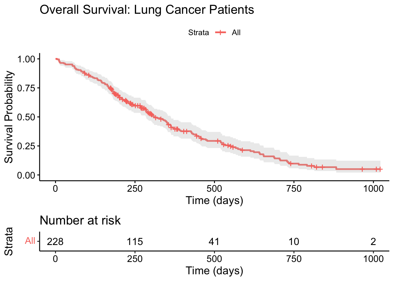
TipHow to Read This Plot

• The solid line shows the estimated survival probability at each time point
• The shaded area is the 95% confidence interval
• The risk table below shows how many patients remain “at risk” (still being followed) at each time point
• Tick marks on the curve indicate censored observations

Median Survival Time

The median survival time is when the survival probability drops to 50%.

surv_median(km_fit)

  strata median lower upper
1    All    310   285   363

The median survival is 310 days, with a 95% CI of 285-363 days.

Survival at Specific Time Points

What’s the probability of surviving 6 months (180 days)? Or 1 year (365 days)?

summary(km_fit, times = c(180, 365, 730))

Call: survfit(formula = Surv(time, status) ~ 1, data = lung)

 time n.risk n.event survival std.err lower 95% CI upper 95% CI
  180    160      63    0.722  0.0298       0.6655        0.783
  365     65      58    0.409  0.0358       0.3447        0.486
  730     13      38    0.116  0.0283       0.0716        0.187

• At 6 months: ~61% survival
• At 1 year: ~41% survival
• At 2 years: ~14% survival

Comparing Groups: Kaplan-Meier by Sex

Now let’s compare survival between males and females. We change the formula to stratify by sex.

km_sex <- survfit(Surv(time, status) ~ sex, data = lung)
print(km_sex)

Call: survfit(formula = Surv(time, status) ~ sex, data = lung)

             n events median 0.95LCL 0.95UCL
sex=Male   138    112    270     212     310
sex=Female  90     53    426     348     550

Females have higher median survival (426 days) compared to males (270 days).

Let’s visualize this difference.

ggsurvplot(
  km_sex,
  data = lung,
  conf.int = TRUE,
  pval = TRUE,
  risk.table = TRUE,
  legend.title = "Sex",
  legend.labs = c("Male", "Female"),
  xlab = "Time (days)",
  ylab = "Survival Probability",
  title = "Survival by Sex"
)

Figure 2

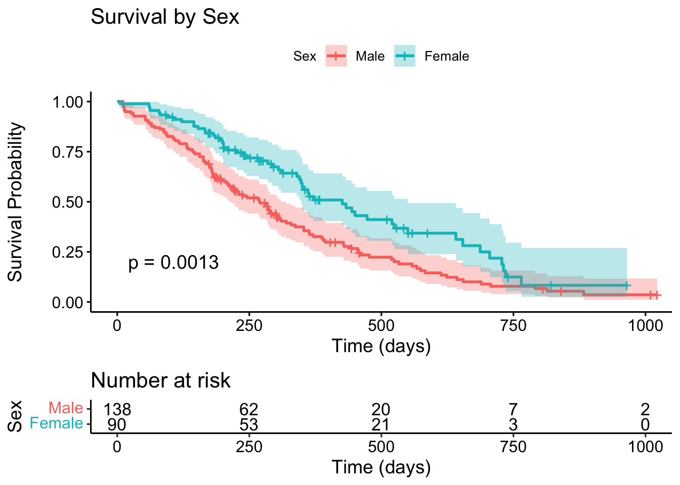
The p-value shown is from the log-rank test (more on this soon). A p-value of 0.0013 suggests a statistically significant difference in survival between males and females.

Comparing Groups: By ECOG Performance Score

ECOG score measures how the disease affects daily living. Let’s see how survival varies by functional status.

First, let’s check the distribution of ECOG scores.

lung |>
  filter(!is.na(ph.ecog)) |>
  count(ph.ecog)

  ph.ecog   n
1       0  63
2       1 113
3       2  50
4       3   1

Most patients have ECOG scores of 0, 1, or 2. Score 3 has only 1 patient, so we’ll filter it out for clearer visualization.

lung_ecog <- lung |>
  filter(!is.na(ph.ecog), ph.ecog != 3)

Now let’s fit the Kaplan-Meier curves by ECOG score.

km_ecog <- survfit(Surv(time, status) ~ ph.ecog, data = lung_ecog)
print(km_ecog)

Call: survfit(formula = Surv(time, status) ~ ph.ecog, data = lung_ecog)

            n events median 0.95LCL 0.95UCL
ph.ecog=0  63     37    394     348     574
ph.ecog=1 113     82    306     268     429
ph.ecog=2  50     44    199     156     288

There’s a clear pattern: higher ECOG scores (worse functional status) have shorter median survival.

ggsurvplot(
  km_ecog,
  data = lung_ecog,
  conf.int = TRUE,
  pval = TRUE,
  risk.table = TRUE,
  legend.title = "ECOG Score",
  xlab = "Time (days)",
  ylab = "Survival Probability",
  title = "Survival by ECOG Performance Score",
  palette = c("#2E9FDF", "#E7B800", "#FC4E07")
)

Figure 3

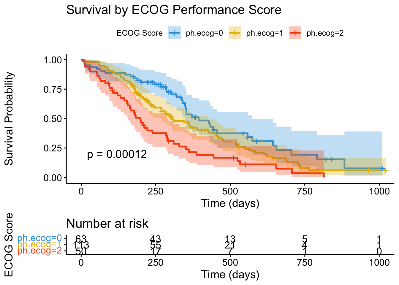
NoteClinical Insight

ECOG performance status is one of the strongest prognostic factors in oncology. Patients who are fully active (ECOG 0) have dramatically better survival than those with limited function (ECOG 2).

The Log-Rank Test

The log-rank test is the standard method for comparing survival curves between groups. It tests the null hypothesis that there’s no difference in survival between groups.

Let’s formally test the difference between males and females.

survdiff(Surv(time, status) ~ sex, data = lung)

Call:
survdiff(formula = Surv(time, status) ~ sex, data = lung)

             N Observed Expected (O-E)^2/E (O-E)^2/V
sex=Male   138      112     91.6      4.55      10.3
sex=Female  90       53     73.4      5.68      10.3

 Chisq= 10.3  on 1 degrees of freedom, p= 0.001 

How to interpret: - N: Number of patients in each group - Observed: Actual number of deaths in each group - Expected: Expected deaths if there were no difference between groups - Chisq: Test statistic (larger = more different from expected) - p-value: Probability of seeing this difference by chance

With p = 0.0013, we reject the null hypothesis. Females have significantly better survival than males.

Let’s also test the ECOG score differences.

survdiff(Surv(time, status) ~ ph.ecog, data = lung_ecog)

Call:
survdiff(formula = Surv(time, status) ~ ph.ecog, data = lung_ecog)

            N Observed Expected (O-E)^2/E (O-E)^2/V
ph.ecog=0  63       37     53.9    5.3014    8.0181
ph.ecog=1 113       82     83.1    0.0144    0.0295
ph.ecog=2  50       44     26.0   12.4571   14.9754

 Chisq= 18  on 2 degrees of freedom, p= 1e-04 

The extremely small p-value (2e-10) confirms that ECOG score is strongly associated with survival.

WarningLog-Rank Limitations

The log-rank test only tells you whether groups differ, not how much they differ. For effect sizes and adjusted comparisons, we need Cox regression.

Cox Proportional Hazards Regression

While Kaplan-Meier curves and log-rank tests are great for comparing groups, they can’t: - Adjust for multiple variables simultaneously - Handle continuous predictors well - Provide a measure of effect size

Cox regression solves all these problems. It models the hazard (instantaneous risk of the event) as a function of predictors.

The Hazard Ratio

The key output of Cox regression is the hazard ratio (HR):

• HR = 1: No effect
• HR > 1: Higher hazard (worse survival)
• HR < 1: Lower hazard (better survival)

For example, HR = 2 means the hazard is doubled - twice the risk of death at any given time.

Simple Cox Model: Effect of Sex

Let’s start with a single predictor: sex.

cox_sex <- coxph(Surv(time, status) ~ sex, data = lung)
summary(cox_sex)

Call:
coxph(formula = Surv(time, status) ~ sex, data = lung)

  n= 228, number of events= 165 

             coef exp(coef) se(coef)      z Pr(>|z|)   
sexFemale -0.5310    0.5880   0.1672 -3.176  0.00149 **
---
Signif. codes:  0 '***' 0.001 '**' 0.01 '*' 0.05 '.' 0.1 ' ' 1

          exp(coef) exp(-coef) lower .95 upper .95
sexFemale     0.588      1.701    0.4237     0.816

Concordance= 0.579  (se = 0.021 )
Likelihood ratio test= 10.63  on 1 df,   p=0.001
Wald test            = 10.09  on 1 df,   p=0.001
Score (logrank) test = 10.33  on 1 df,   p=0.001

Let’s break down the key output:

coef: The log hazard ratio. Negative means lower hazard (better survival).

exp(coef): The hazard ratio itself. For females: HR = 0.59.

Interpretation: Females have 59% the hazard of males, or equivalently, 41% lower risk of death at any given time.

p-value: 0.00149 confirms this is statistically significant.

We can extract just the hazard ratio and CI more cleanly.

exp(coef(cox_sex))

sexFemale 
0.5880028 

exp(confint(cox_sex))

              2.5 %    97.5 %
sexFemale 0.4237178 0.8159848

TipInterpreting Hazard Ratios

HR = 0.59 for females means: at any point in time, a female patient has about 59% the hazard (risk of death) compared to a male patient. This is a 41% reduction in hazard.

Multiple Cox Regression

Now let’s build a model with multiple predictors: sex, age, and ECOG score.

cox_multi <- coxph(
  Surv(time, status) ~ sex + age + ph.ecog,
  data = lung_ecog
)
summary(cox_multi)

Call:
coxph(formula = Surv(time, status) ~ sex + age + ph.ecog, data = lung_ecog)

  n= 226, number of events= 163 

               coef exp(coef)  se(coef)      z Pr(>|z|)    
sexFemale -0.545631  0.579476  0.168229 -3.243  0.00118 ** 
age        0.010777  1.010836  0.009312  1.157  0.24713    
ph.ecog1   0.409836  1.506571  0.199606  2.053  0.04005 *  
ph.ecog2   0.902321  2.465318  0.228092  3.956 7.62e-05 ***
ph.ecog3         NA        NA  0.000000     NA       NA    
---
Signif. codes:  0 '***' 0.001 '**' 0.01 '*' 0.05 '.' 0.1 ' ' 1

          exp(coef) exp(-coef) lower .95 upper .95
sexFemale    0.5795     1.7257    0.4167    0.8058
age          1.0108     0.9893    0.9926    1.0295
ph.ecog1     1.5066     0.6638    1.0188    2.2279
ph.ecog2     2.4653     0.4056    1.5766    3.8550
ph.ecog3         NA         NA        NA        NA

Concordance= 0.635  (se = 0.025 )
Likelihood ratio test= 28.94  on 4 df,   p=8e-06
Wald test            = 28.6  on 4 df,   p=9e-06
Score (logrank) test = 29.68  on 4 df,   p=6e-06

Let’s extract the hazard ratios for all variables.

library(broom)

tidy(cox_multi, exponentiate = TRUE, conf.int = TRUE) |>
  select(term, estimate, conf.low, conf.high, p.value) |>
  mutate(across(where(is.numeric), ~round(., 3)))

# A tibble: 5 × 5
  term      estimate conf.low conf.high p.value
  <chr>        <dbl>    <dbl>     <dbl>   <dbl>
1 sexFemale    0.579    0.417     0.806   0.001
2 age          1.01     0.993     1.03    0.247
3 ph.ecog1     1.51     1.02      2.23    0.04 
4 ph.ecog2     2.46     1.58      3.86    0    
5 ph.ecog3    NA       NA        NA      NA    

Key findings: - Sex (Female): HR = 0.57, meaning 43% lower hazard than males (adjusted) - Age: HR = 1.01 per year - modest effect (1% higher hazard per year of age) - ECOG 1: HR = 1.58 - 58% higher hazard than ECOG 0 - ECOG 2: HR = 2.68 - 168% higher hazard than ECOG 0

Forest Plot of Hazard Ratios

A forest plot is a clean way to visualize all hazard ratios.

ggforest(cox_multi, data = lung_ecog)

Figure 4

This plot shows: - Point estimates (squares) - 95% confidence intervals (horizontal lines) - Reference line at HR = 1 (no effect) - P-values for each variable

Model Diagnostics: Proportional Hazards Assumption

Cox regression assumes that hazard ratios remain constant over time (the “proportional hazards” assumption). We should test this.

The cox.zph() function tests this assumption using Schoenfeld residuals.

ph_test <- cox.zph(cox_multi)
print(ph_test)

        chisq df    p
sex     2.440  1 0.12
age     0.163  1 0.69
ph.ecog 2.871  2 0.24
GLOBAL  4.992  4 0.29

How to interpret: - Each row tests one variable - GLOBAL tests the overall model - p > 0.05 means the assumption is satisfied

All p-values are well above 0.05, so the proportional hazards assumption holds. Our model is valid.

We can also visualize the Schoenfeld residuals.

ggcoxzph(ph_test)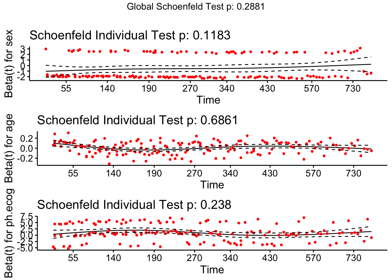

Figure 5

NoteWhat If PH Assumption Fails?

If a variable violates proportional hazards (curved line, significant p-value), you can: 1. Stratify by that variable: coxph(Surv(...) ~ x + strata(z), data) 2. Include a time-interaction: coxph(Surv(...) ~ x + x:log(time), data) 3. Use time-varying coefficients

Summary

In this tutorial, we covered the essentials of survival analysis:

Concept	Description	R Function
Survival object	Pairs time with censoring status	Surv()
Kaplan-Meier	Non-parametric survival estimate	survfit()
Log-rank test	Compare survival between groups	survdiff()
Cox regression	Model hazard as function of predictors	coxph()
Hazard ratio	Effect size (HR > 1 = worse survival)	exp(coef())
PH assumption	Test proportional hazards	cox.zph()

Quick Reference

NoteSurvival Analysis Workflow

1. Create survival object

surv_obj <- Surv(time = df$time, event = df$status)

2. Kaplan-Meier curve

km_fit <- survfit(Surv(time, status) ~ group, data = df)
ggsurvplot(km_fit, data = df, pval = TRUE)

3. Log-rank test

survdiff(Surv(time, status) ~ group, data = df)

4. Cox regression

cox_fit <- coxph(Surv(time, status) ~ x1 + x2, data = df)
summary(cox_fit)
ggforest(cox_fit, data = df)

5. Check proportional hazards

cox.zph(cox_fit)

Frequently Asked Questions

Q: What’s the difference between survival probability and hazard?

Survival probability S(t) is the probability of surviving beyond time t. Hazard h(t) is the instantaneous risk of the event at time t, given survival up to that point. They’re related: higher hazard means survival probability decreases faster.

Q: How do I handle left-censored or interval-censored data?

The survival package supports these with Surv(time1, time2, type = "interval"). However, Kaplan-Meier assumes right-censoring only. For other censoring types, consider parametric models or the icenReg package.

Q: What sample size do I need for survival analysis?

A common rule of thumb: you need about 10 events per predictor variable in Cox regression. With 3 predictors, aim for at least 30 events. The powerSurvEpi package can help with formal power calculations.

Q: Can I use survival analysis for competing risks?

Yes! When subjects can experience multiple types of events (e.g., death from cancer vs. death from other causes), use the cmprsk package for competing risk analysis.

Q: How do I handle time-varying covariates?

If a predictor changes over time (e.g., treatment status), you need the counting process format: Surv(start, stop, event). Split each subject’s data at times when covariates change.

Q: What’s the difference between Cox regression and parametric survival models?

Cox regression is semi-parametric - it makes no assumptions about the baseline hazard shape. Parametric models (Weibull, exponential, log-normal) assume a specific hazard function. Cox is more flexible; parametric models are more efficient when assumptions are met.

Q: How do I handle missing data in survival analysis?

The easiest approach is complete case analysis, but this can bias results. Multiple imputation with the mice package works for covariates. For missing survival times or censoring indicators, the problem is more complex - consider sensitivity analyses.

---

Further Reading

• survival Package Documentation - Comprehensive reference
• survminer Package - Beautiful survival plots
• Survival Analysis in R (Emily Zabor) - Excellent tutorial
• Applied Survival Analysis Using R (Moore, 2016) - Textbook
• Therneau & Grambsch: Modeling Survival Data - The definitive reference

Related Posts

• Introduction to Mixed Effects Models in R
• Introduction to Empirical Bayes in R
• How to logistic regression in R
• How to linear regression basics in R