How to use geom_label() in R

Learn how to use geom_label() in R with practical examples. Step-by-step guide with code you can copy and run immediately.

Introduction

The geom_label() function in ggplot2 creates text labels with a rectangular background, making them stand out clearly on plots. Unlike geom_text(), these labels have a solid background that improves readability, especially when text overlaps with data points or complex backgrounds.

Getting Started

library(tidyverse)
library(palmerpenguins)

Example 1: Basic Usage

The Problem

We want to add clear, readable labels to highlight specific data points on a scatter plot. Regular text can be hard to read when it overlaps with plot elements.

Step 1: Create a basic scatter plot

Let’s start with a simple plot showing the relationship between penguin bill length and depth.

p1 <- penguins |>
  ggplot(aes(x = bill_length_mm, y = bill_depth_mm)) +
  geom_point(alpha = 0.7)

p1

This creates our foundation scatter plot with all penguin measurements plotted as points.

Step 2: Add basic labels

Now we’ll add labels to identify different penguin species using geom_label().

p1 + 
  geom_label(aes(label = species), 
            alpha = 0.8,
            size = 3)

The labels now appear with white backgrounds, making them clearly readable against any background elements.

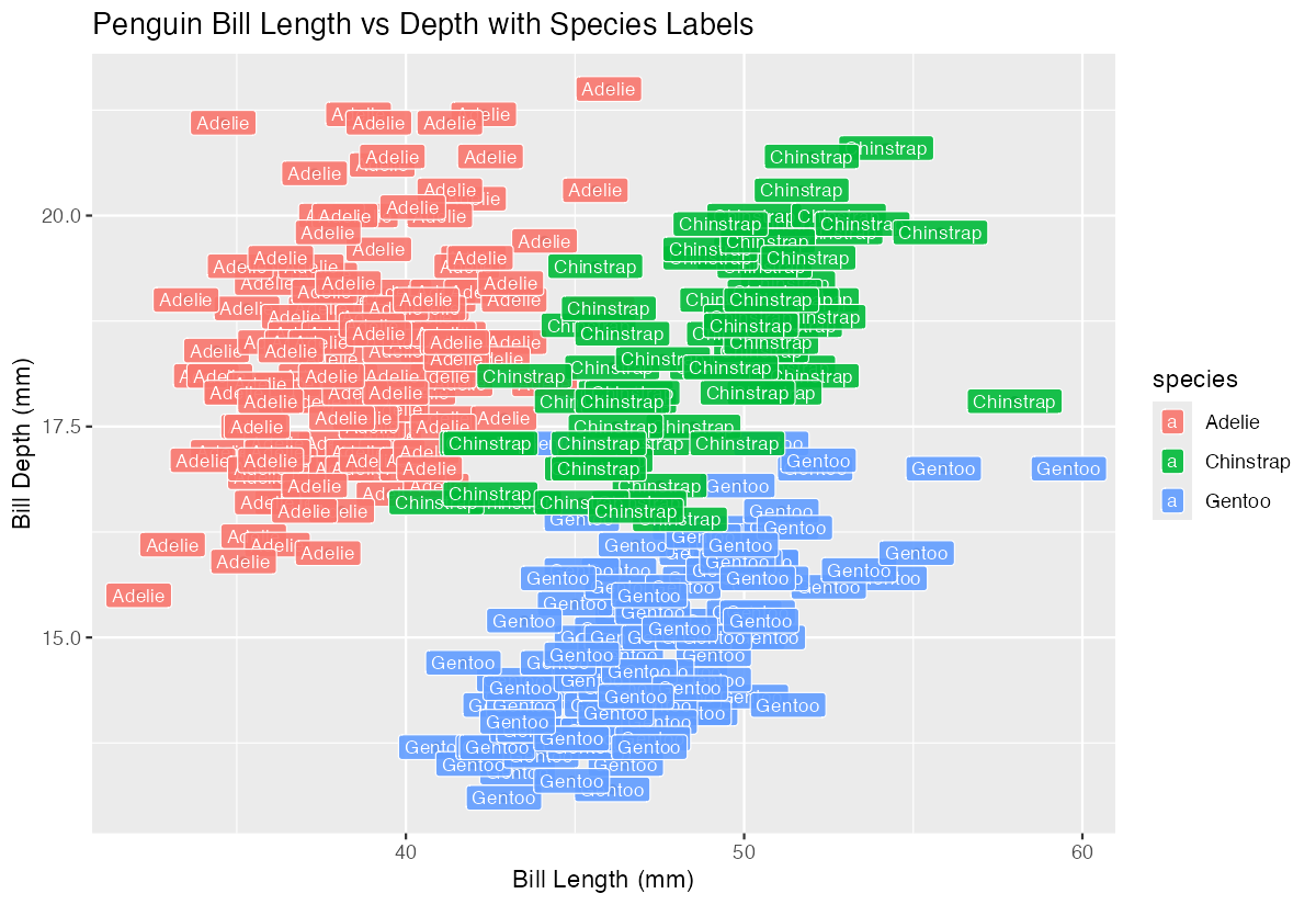
Step 3: Customize label appearance

We can improve the labels by adjusting colors and positioning.

penguins |>
  ggplot(aes(x = bill_length_mm, y = bill_depth_mm)) +
  geom_point(alpha = 0.5) +
  geom_label(aes(label = species, fill = species), 
            color = "white",
            size = 3,
            alpha = 0.9)

Now each species has its own colored background with white text for better contrast.

Scatter plot in R using geom_label() in ggplot2 showing penguin bill length versus bill depth with colored species labels on rectangular backgrounds from the palmerpenguins dataset

Example 2: Practical Application

The Problem

We need to create a summary visualization showing average bill measurements by species, with clearly labeled data points. This is common when presenting findings to stakeholders who need to quickly identify key values.

Step 1: Calculate species averages

First, let’s compute the mean bill measurements for each penguin species.

penguin_summary <- penguins |>
  group_by(species) |>
  summarise(
    avg_length = mean(bill_length_mm, na.rm = TRUE),
    avg_depth = mean(bill_depth_mm, na.rm = TRUE),
    .groups = 'drop'
  )

penguin_summary

This gives us clean summary data with average measurements for each species.

Step 2: Create the base visualization

Now we’ll plot these averages as distinct points for each species.

p2 <- penguin_summary |>
  ggplot(aes(x = avg_length, y = avg_depth, color = species)) +
  geom_point(size = 4) +
  theme_minimal()

p2

We have a clean plot showing the three species as colored points representing their average measurements.

Step 3: Add informative labels with values

Let’s add labels that show both the species name and the exact measurements.

penguin_summary |>
  mutate(label_text = paste0(species, "\n(", 
                            round(avg_length, 1), "mm, ",
                            round(avg_depth, 1), "mm)")) |>
  ggplot(aes(x = avg_length, y = avg_depth)) +
  geom_point(aes(color = species), size = 4) +
  geom_label(aes(label = label_text, fill = species),
            color = "white",
            size = 3.5,
            nudge_y = 0.5) +
  theme_minimal()

The labels now display species names with exact measurements, positioned slightly above each point for clarity.

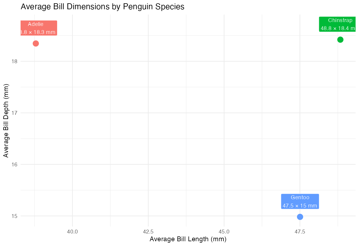
Step 4: Polish the final visualization

Finally, let’s add proper titles and remove the legend since labels provide the information.

penguin_summary |>
  mutate(label_text = paste0(species, "\n", 
                            round(avg_length, 1), " × ",
                            round(avg_depth, 1), " mm")) |>
  ggplot(aes(x = avg_length, y = avg_depth)) +
  geom_point(aes(color = species), size = 4) +
  geom_label(aes(label = label_text, fill = species),
            color = "white", size = 3.2, nudge_y = 0.3) +
  labs(title = "Average Bill Dimensions by Penguin Species",
       x = "Average Bill Length (mm)",
       y = "Average Bill Depth (mm)") +
  theme_minimal() +
  theme(legend.position = "none")

This creates a publication-ready visualization with clear, informative labels that eliminate the need for a separate legend.

Summary plot in R using geom_label() in ggplot2 showing average bill length and depth dimensions for each penguin species with informative rectangular labels from the palmerpenguins dataset

Summary

• geom_label() creates text labels with solid backgrounds for improved readability
• Use aes(label = column_name) to specify which data to display in labels
  
• Customize appearance with fill, color, size, and alpha parameters
• Use nudge_x and nudge_y to position labels away from overlapping elements

• Combine with paste0() to create multi-line or formatted label text

Related Posts

• How to use geom_point() in R
• How to use geom_area() in R
• How to use geom_tile() in R
• How to use select() in R
• How to use mutate() in R