How to use geom_line() in R
Introduction
The geom_line() function in ggplot2 creates line graphs by connecting data points with straight lines. It’s perfect for visualizing trends over time, showing relationships between continuous variables, or displaying changes in values across ordered categories.
Getting Started
library(tidyverse)
library(palmerpenguins)
Example 1: Basic Line Plot
The Problem
We want to create a simple line plot showing how penguin body mass varies across different flipper lengths. This will help us understand the basic relationship between these two continuous variables.
Step 1: Prepare the data
We’ll start by examining our dataset and selecting the variables we need.
# Look at the penguins data structure
glimpse(penguins)

# Create a basic line plot
penguins |>
  filter(!is.na(flipper_length_mm), !is.na(body_mass_g))
This gives us a clean dataset with no missing values for our variables of interest.
Step 2: Create the basic line plot
Now we’ll create our first line plot using the default settings.
penguins |>
  filter(!is.na(flipper_length_mm), !is.na(body_mass_g)) |>
  ggplot(aes(x = flipper_length_mm, y = body_mass_g)) +
  geom_line()
The plot connects all points in order of the x-axis values, creating a zigzag pattern that shows the data distribution.
Step 3: Improve the plot appearance
Let’s add proper labels and styling to make the plot more professional.
penguins |>
  filter(!is.na(flipper_length_mm), !is.na(body_mass_g)) |>
  ggplot(aes(x = flipper_length_mm, y = body_mass_g)) +
  geom_line(color = "steelblue", linewidth = 0.8) +
  labs(title = "Penguin Body Mass vs Flipper Length",
       x = "Flipper Length (mm)",
       y = "Body Mass (g)")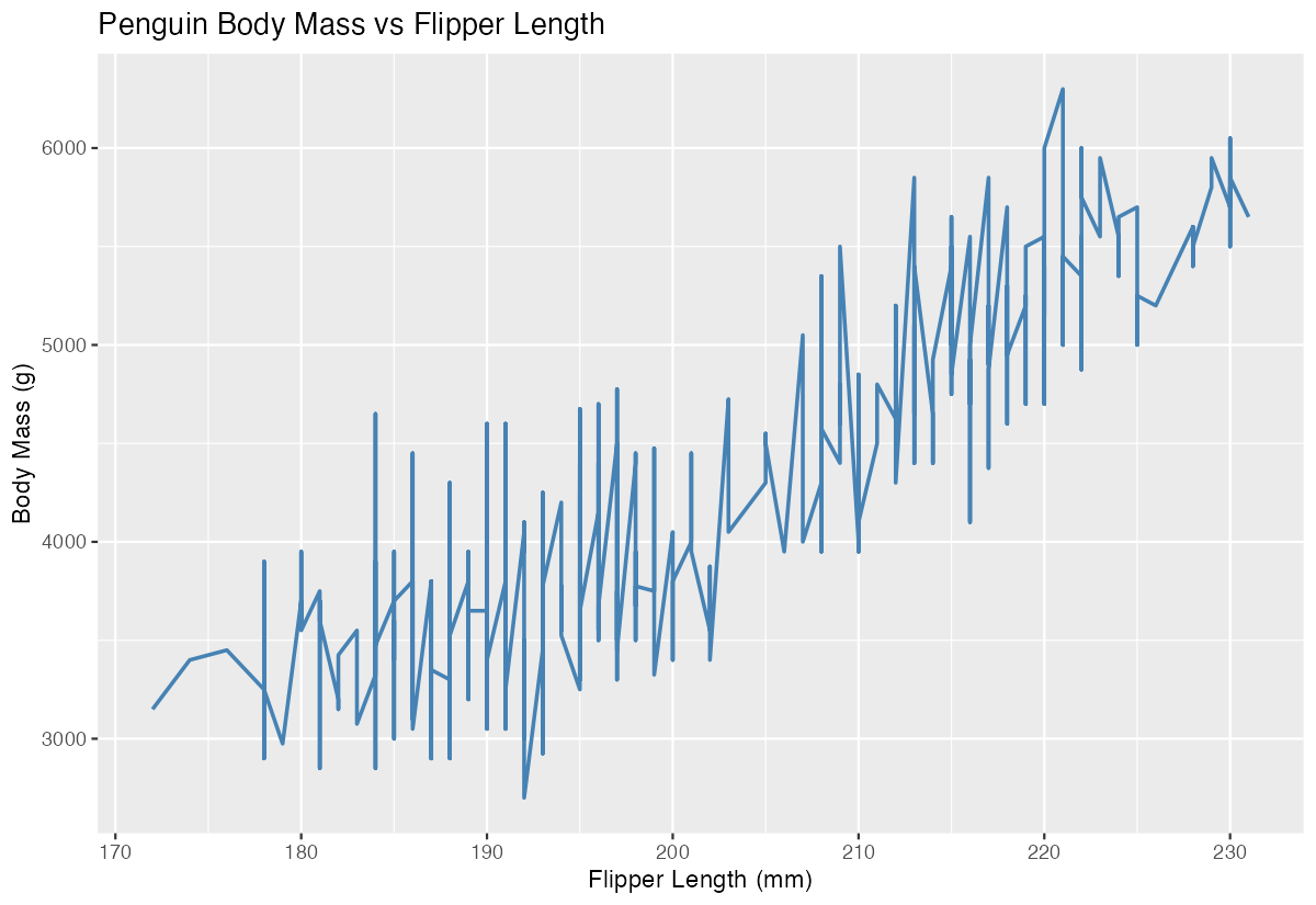
The result is a clean, styled line plot that clearly shows the relationship between flipper length and body mass.
Example 2: Time Series Analysis
The Problem
We want to analyze car performance trends over time using the mtcars dataset. Specifically, we’ll look at how average miles per gallon (mpg) varies across different numbers of cylinders, treating cylinders as a sequential variable to demonstrate time-series-like visualization.
Step 1: Aggregate the data
First, we need to calculate average mpg for each cylinder group.
mpg_by_cylinders <- mtcars |>
  group_by(cyl) |>
  summarise(avg_mpg = mean(mpg),
            count = n()) |>
  arrange(cyl)

print(mpg_by_cylinders)
This creates a summary table showing average fuel efficiency for 4, 6, and 8-cylinder cars.
Step 2: Create the trend line
Now we’ll visualize this trend using a line plot with enhanced styling.
mpg_by_cylinders |>
  ggplot(aes(x = cyl, y = avg_mpg)) +
  geom_line(color = "darkred", size = 1.2) +
  geom_point(size = 3, color = "darkred")
The combination of line and points clearly shows the declining trend in fuel efficiency as cylinder count increases.
Step 3: Add context and formatting
Let’s enhance the plot with better scaling and annotations.
mpg_by_cylinders |>
  ggplot(aes(x = cyl, y = avg_mpg)) +
  geom_line(color = "darkred", linewidth = 1.2) +
  geom_point(size = 3, color = "darkred") +
  scale_x_continuous(breaks = c(4, 6, 8)) +
  labs(title = "Average MPG by Number of Cylinders",
       x = "Number of Cylinders",
       y = "Average Miles per Gallon") +
  theme_minimal()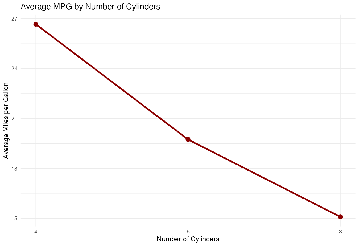
The final plot provides a clear, professional visualization of the relationship between engine size and fuel efficiency.
Step 4: Add multiple lines for comparison
We can extend this analysis by adding transmission type as a grouping variable.
mtcars |>
  mutate(transmission = ifelse(am == 0, "Automatic", "Manual")) |>
  group_by(cyl, transmission) |>
  summarise(avg_mpg = mean(mpg), .groups = "drop") |>
  ggplot(aes(x = cyl, y = avg_mpg, color = transmission)) +
  geom_line(linewidth = 1.2) +
geom_point(size = 3)![]()
This creates two separate trend lines, allowing us to compare fuel efficiency patterns between automatic and manual transmissions across different engine sizes.
Summary
geom_line()connects data points with straight lines, ideal for showing trends and relationships- Always filter out missing values before creating line plots to avoid gaps or errors
- Combine
geom_line()withgeom_point()to highlight individual data points along the trend - Use
aes(color = variable)to create multiple lines for different groups in your data Enhance readability with proper labels, colors, and themes for professional-looking visualizations