How to use geom_ribbon() in R
Introduction
The geom_ribbon() function in ggplot2 creates filled areas between two y-values, making it perfect for visualizing confidence intervals, error bands, or ranges in data. It’s commonly used in statistical plots to show uncertainty around predictions or to highlight areas between curves.
Getting Started
library(tidyverse)
library(palmerpenguins)
Example 1: Basic Usage
The Problem
We want to create a simple ribbon plot showing the range between minimum and maximum penguin body mass values across different flipper lengths. This will help us understand the spread of body mass measurements.
Step 1: Prepare the data
First, we’ll calculate summary statistics for body mass by flipper length.
penguin_summary <- penguins |>
  filter(!is.na(body_mass_g), !is.na(flipper_length_mm)) |>
  group_by(flipper_length_mm) |>
  summarise(
    min_mass = min(body_mass_g),
    max_mass = max(body_mass_g),
    .groups = 'drop'
  )
This creates a dataset with minimum and maximum body mass values for each flipper length.
Step 2: Create the basic ribbon plot
Now we’ll use geom_ribbon() to visualize the range between minimum and maximum values.
ggplot(penguin_summary, aes(x = flipper_length_mm)) +
  geom_ribbon(aes(ymin = min_mass, ymax = max_mass),
              alpha = 0.3, fill = "blue") +
  labs(x = "Flipper Length (mm)",
       y = "Body Mass (g)")
The ribbon shows the full range of body mass values, with the shaded area representing the spread between minimum and maximum values.
Step 3: Add a center line
Let’s enhance the plot by adding the mean body mass as a line through the ribbon.
penguin_summary <- penguin_summary |>
  left_join(
    penguins |>
      group_by(flipper_length_mm) |>
      summarise(mean_mass = mean(body_mass_g, na.rm = TRUE))
  )
This adds the mean body mass for each flipper length to our summary data.
Step 4: Complete the ribbon plot
Now we’ll create the final plot with both the ribbon and center line.
ggplot(penguin_summary, aes(x = flipper_length_mm)) +
  geom_ribbon(aes(ymin = min_mass, ymax = max_mass),
              alpha = 0.3, fill = "steelblue") +
  geom_line(aes(y = mean_mass), color = "darkblue", linewidth = 1) +
  labs(title = "Penguin Body Mass Range by Flipper Length",
       subtitle = "Ribbon shows min-max range, line shows mean",
       x = "Flipper Length (mm)", y = "Body Mass (g)") +
  theme_minimal()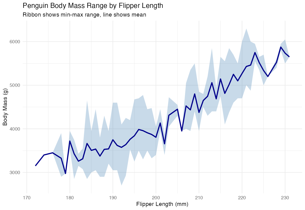
The completed plot shows both the range (ribbon) and average (line) of body mass across flipper lengths.
Example 2: Practical Application
The Problem
We need to create a confidence interval plot showing the relationship between car weight and fuel efficiency. This is a common scenario in data analysis where we want to show both the predicted line and the uncertainty around our predictions.
Step 1: Fit a model and generate predictions
First, we’ll create a linear model and generate predictions with confidence intervals.
model <- lm(mpg ~ wt, data = mtcars)
new_data <- data.frame(wt = seq(min(mtcars$wt), max(mtcars$wt),
                               length.out = 100))
predictions <- predict(model, new_data, interval = "confidence")
This creates smooth predictions across the weight range with 95% confidence intervals.
Step 2: Combine predictions with original data
Next, we’ll combine our predictions into a single data frame for plotting.
plot_data <- data.frame(
  wt = new_data$wt,
  fit = predictions[,"fit"],
  lower = predictions[,"lwr"],
  upper = predictions[,"upr"]
)
Now we have all the necessary components: the fitted line and confidence bounds.
Step 3: Create the confidence interval plot
Finally, we’ll create a professional-looking plot with the ribbon showing confidence intervals.
ggplot() +
  geom_ribbon(data = plot_data,
              aes(x = wt, ymin = lower, ymax = upper),
              alpha = 0.2, fill = "red") +
  geom_line(data = plot_data, aes(x = wt, y = fit),
            color = "red", size = 1) +
  geom_point(data = mtcars, aes(x = wt, y = mpg))
The ribbon shows the confidence interval around our regression line, with actual data points overlaid.
Step 4: Polish the visualization
Let’s add proper labels and styling to make the plot publication-ready.
ggplot() +
  geom_ribbon(data = plot_data,
              aes(x = wt, ymin = lower, ymax = upper),
              alpha = 0.2, fill = "red") +
  geom_line(data = plot_data, aes(x = wt, y = fit),
            color = "red", linewidth = 1) +
  geom_point(data = mtcars, aes(x = wt, y = mpg)) +
  labs(title = "Car Weight vs Fuel Efficiency",
       subtitle = "Linear regression with 95% confidence ribbon",
       x = "Weight (1000 lbs)", y = "Miles per Gallon") +
  theme_classic()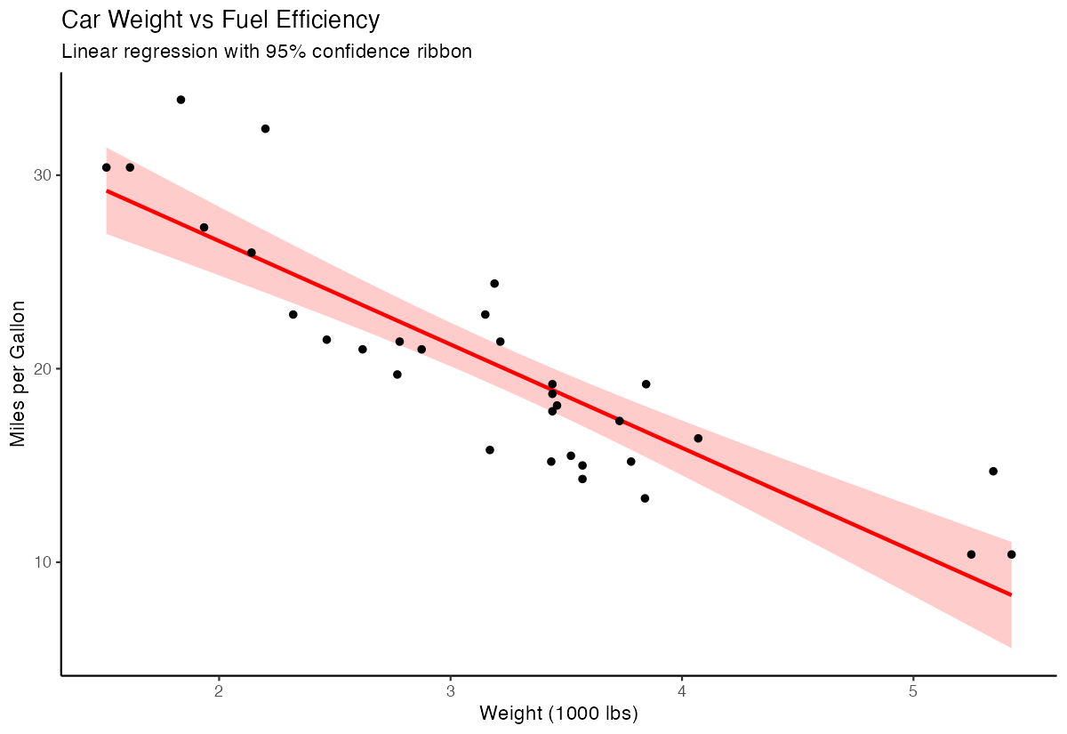
The final plot clearly shows the relationship between weight and fuel efficiency with confidence bounds.
Summary
geom_ribbon()requiresyminandymaxaesthetics to define the ribbon boundaries- Use
alphaparameter to control transparency and avoid overwhelming other plot elements - Combine ribbons with
geom_line()orgeom_point()to show central tendencies alongside ranges - Common applications include confidence intervals, prediction bands, and min/max ranges
Always ensure your data is properly sorted by x-values for smooth ribbon appearance