How to use geom_smooth() in R
Introduction
The geom_smooth() function in ggplot2 adds smooth trend lines to scatter plots, helping reveal underlying patterns in your data. Use it when you want to visualize relationships between variables without being distracted by individual data point variations.
Getting Started
library(tidyverse)
library(palmerpenguins)
Example 1: Basic Usage
The Problem
You have a scatter plot of penguin bill length versus bill depth, but the individual points make it hard to see the overall relationship pattern.
Step 1: Create a basic scatter plot
First, let’s create a simple scatter plot to see our data.
penguins |>
  ggplot(aes(x = bill_length_mm, y = bill_depth_mm)) +
  geom_point()
This shows all the individual penguin measurements as points, but the trend isn’t immediately clear.
Step 2: Add a smooth trend line
Now we’ll add a smooth line to reveal the underlying pattern.
penguins |>
  ggplot(aes(x = bill_length_mm, y = bill_depth_mm)) +
  geom_point() +
  geom_smooth()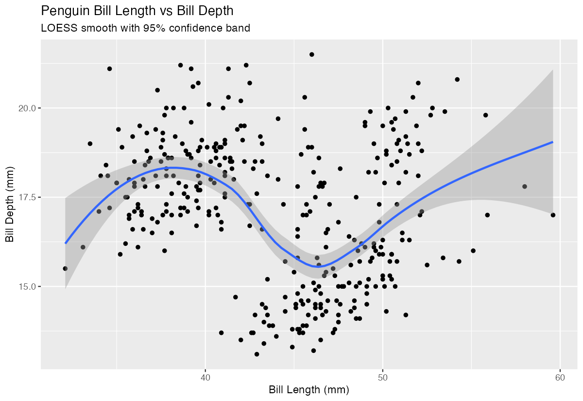
The gray ribbon shows the confidence interval around the smooth blue trend line, revealing a slight negative relationship.
Step 3: Remove confidence bands
Sometimes the confidence interval can be distracting, so we can remove it.
penguins |>
  ggplot(aes(x = bill_length_mm, y = bill_depth_mm)) +
  geom_point() +
  geom_smooth(se = FALSE)
Setting se = FALSE removes the gray confidence band, leaving just the clean trend line.
Example 2: Practical Application
The Problem
You’re analyzing car performance data and want to understand how engine displacement affects fuel efficiency. You also want to compare different smoothing methods to see which reveals the pattern most clearly.
Step 1: Explore the basic relationship
Let’s start by examining the relationship between engine size and miles per gallon.
mtcars |>
  ggplot(aes(x = disp, y = mpg)) +
  geom_point() +
  geom_smooth()
This reveals a clear negative relationship - larger engines tend to have lower fuel efficiency.
Step 2: Try different smoothing methods
The default uses LOESS smoothing, but we can try a linear model instead.
mtcars |>
  ggplot(aes(x = disp, y = mpg)) +
  geom_point() +
  geom_smooth(method = "lm")
Using method = "lm" fits a straight line, which might be more appropriate for this linear-looking relationship.
Step 3: Compare multiple methods
We can overlay different smoothing methods to compare their approaches.
mtcars |>
  ggplot(aes(x = disp, y = mpg)) +
  geom_point() +
  geom_smooth(method = "lm", color = "red", se = FALSE) +
  geom_smooth(method = "loess", color = "blue", se = FALSE)
The red linear line and blue LOESS curve show similar patterns, helping confirm the relationship’s nature.
Step 4: Add grouping by categories
Let’s see how transmission type affects the relationship pattern.
mtcars |>
  ggplot(aes(x = disp, y = mpg, color = factor(am))) +
  geom_point() +
geom_smooth(method = "lm", se = FALSE)![]()
This creates separate trend lines for automatic (0) and manual (1) transmissions, revealing different efficiency patterns.
Step 5: Customize the appearance
Finally, let’s make the plot more presentation-ready with better styling.
mtcars |>
  ggplot(aes(x = disp, y = mpg)) +
  geom_point(alpha = 0.6) +
  geom_smooth(color = "darkblue", fill = "lightblue") +
  labs(x = "Engine Displacement", y = "Miles per Gallon")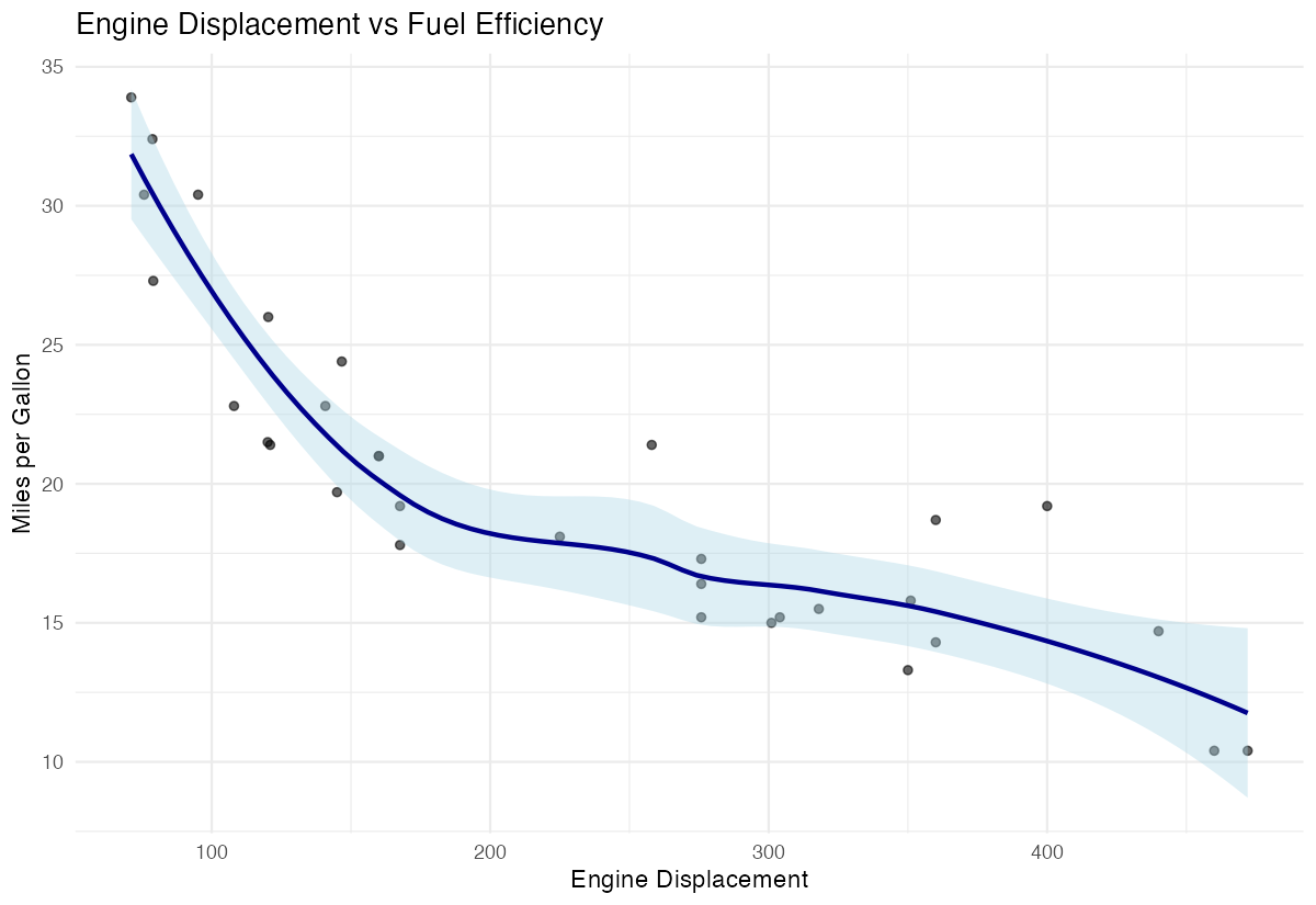
This adds transparency to points and custom colors to the smooth line and confidence interval.
Summary
geom_smooth()adds trend lines to help identify patterns in scatter plots- Use
se = FALSEto remove confidence intervals when they’re distracting - The
methodparameter lets you choose between LOESS (default), linear models (“lm”), and other smoothing approaches - Group-wise smoothing with color aesthetics reveals how relationships vary across categories
Combine with customized colors and transparency for publication-ready visualizations