How to use theme_minimal() in R
Introduction
The theme_minimal() function in ggplot2 creates clean, professional-looking plots by removing unnecessary visual clutter like background colors and grid lines. This theme is perfect when you want your data to stand out without distracting design elements, making it ideal for reports, presentations, and publications.
Getting Started
library(tidyverse)
library(palmerpenguins)
Example 1: Basic Usage
The Problem
Default ggplot2 themes can look cluttered with gray backgrounds and excessive grid lines. We need a cleaner approach to showcase our penguin data effectively.
Step 1: Create a basic scatter plot
Let’s start with a standard scatter plot to see the default appearance.
basic_plot <- penguins |>
  ggplot(aes(x = bill_length_mm, y = bill_depth_mm)) +
  geom_point(aes(color = species))

basic_plot
This creates a scatter plot with the default gray theme, which includes a gray background and white grid lines.
Step 2: Apply theme_minimal()
Now we’ll apply the minimal theme to clean up the appearance.
minimal_plot <- basic_plot +
  theme_minimal()

minimal_plot
The plot now has a clean white background with subtle gray grid lines, making the data points more prominent.
Step 3: Add informative labels
Let’s complete the visualization with proper titles and labels.
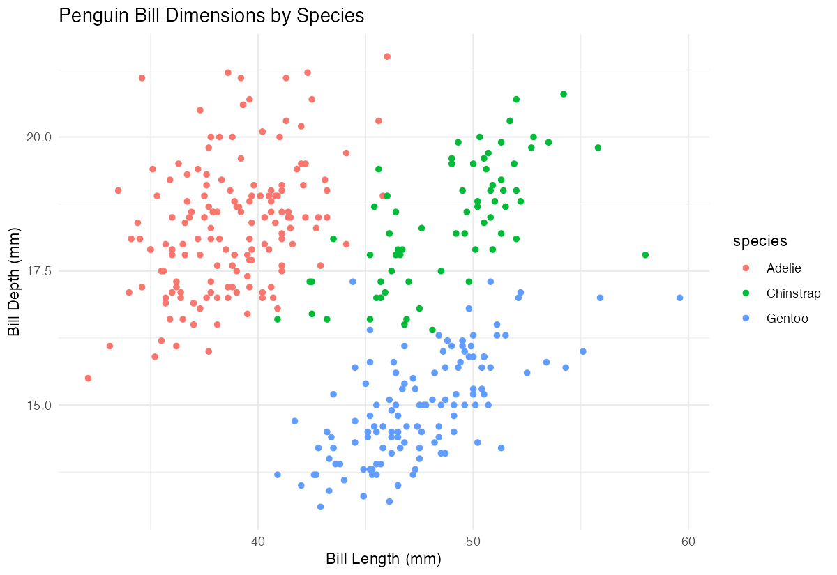
final_plot <- minimal_plot +
  labs(
    title = "Penguin Bill Dimensions by Species",
    x = "Bill Length (mm)",
    y = "Bill Depth (mm)"
  )

final_plot
The minimal theme ensures our labels and data remain the focus without visual distractions.
Example 2: Practical Application
The Problem
You’re creating a dashboard showing car performance metrics for a business presentation. The default theme looks unprofessional, and you need multiple plots with consistent, clean styling that won’t distract from the data insights.
Step 1: Create the base visualization
We’ll start with a multi-faceted plot showing the relationship between car weight and fuel efficiency.
car_plot <- mtcars |>
  mutate(transmission = ifelse(am == 1, "Manual", "Automatic")) |>
  ggplot(aes(x = wt, y = mpg)) +
  geom_point(aes(color = factor(cyl)), size = 3)

car_plot
This creates our base plot with colored points representing different cylinder counts.
Step 2: Apply minimal theme with customizations
Now we’ll add the minimal theme and customize it for professional presentation.
styled_plot <- car_plot +
  theme_minimal() +
  theme(
    plot.title = element_text(size = 14, face = "bold"),
    legend.position = "bottom"
  )

styled_plot
The minimal theme provides a clean foundation, while our customizations enhance readability for presentations.
Step 3: Add professional labels and faceting
Let’s complete the visualization with clear labels and faceting by transmission type.
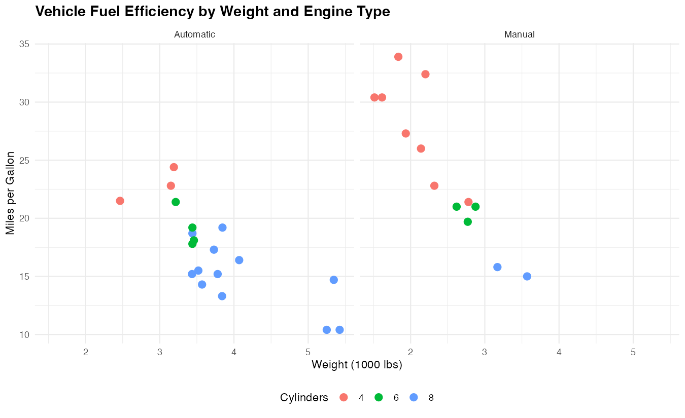
dashboard_plot <- styled_plot +
  facet_wrap(~transmission) +
  labs(
    title = "Vehicle Fuel Efficiency by Weight and Engine Type",
    x = "Weight (1000 lbs)",
    y = "Miles per Gallon",
    color = "Cylinders"
  )

dashboard_plot
The result is a professional, publication-ready visualization that clearly communicates the data relationships.
Step 4: Create a consistent theme for multiple plots
For dashboard consistency, save your theme customizations as a reusable function.
my_minimal_theme <- function() {
  theme_minimal() +
  theme(
    plot.title = element_text(size = 14, face = "bold"),
    legend.position = "bottom",
    strip.text = element_text(face = "bold")
  )
}
Now you can apply this consistent styling across all your dashboard plots with a simple + my_minimal_theme().
Summary
theme_minimal()removes visual clutter by eliminating gray backgrounds and reducing grid line prominence- It works perfectly for professional presentations, reports, and publications where data clarity is paramount
- The theme can be easily customized by adding additional
theme()elements for specific styling needs - Consistent application across multiple plots creates cohesive, professional-looking dashboards
Always combine with clear labels and titles to maximize the impact of your clean, minimal design