How to Compute Pearson Correlation of Multiple Variables
Introduction
The Pearson correlation coefficient measures the linear relationship between variables, ranging from -1 to 1. When working with datasets containing multiple variables, computing correlations between all pairs helps identify relationships and patterns. This is essential for exploratory data analysis and feature selection in statistical modeling.
Getting Started
library(tidyverse)
library(palmerpenguins)
Example 1: Basic Correlation Matrix
The Problem
We need to calculate correlations between all numeric variables in the penguins dataset. This will show us which measurements are most strongly related to each other.
Step 1: Select Numeric Variables
First, we’ll extract only the numeric columns from our dataset.
penguins_numeric <- penguins |>
  select(bill_length_mm, bill_depth_mm,
         flipper_length_mm, body_mass_g) |>
  na.omit()
This creates a clean dataset with four numeric variables and removes any missing values.
Step 2: Create Basic Correlation Matrix
Now we’ll compute the correlation matrix using the base R cor() function.
correlation_matrix <- cor(penguins_numeric,
                         method = "pearson")
print(correlation_matrix)
The result shows correlations between all variable pairs, with 1.0 on the diagonal (each variable perfectly correlates with itself).
Step 3: Round for Better Readability
Let’s round the values to make them easier to interpret.
correlation_matrix_rounded <- correlation_matrix |>
  round(3)
print(correlation_matrix_rounded)
Now we can easily see that flipper length and body mass have a strong positive correlation (around 0.871).
Example 2: Practical Application
The Problem
A marine biologist wants to understand which penguin measurements are most related to body mass for predicting penguin health. They also need to visualize these relationships and handle the analysis by species groups.
Step 1: Compute Correlations with Body Mass
We’ll focus specifically on correlations with body mass as our target variable.
body_mass_correlations <- penguins |>
  select(bill_length_mm, bill_depth_mm,
         flipper_length_mm, body_mass_g) |>
  cor(use = "complete.obs") |>
  as.data.frame() |>
  select(body_mass_g)
This extracts only the body mass column from the correlation matrix, showing how each measurement relates to penguin weight.
Step 2: Create Correlation by Species
Different penguin species might show different correlation patterns.
species_correlations <- penguins |>
  group_by(species) |>
  summarise(
    bill_length_cor = cor(bill_length_mm, body_mass_g, use = "complete.obs"),
    bill_depth_cor = cor(bill_depth_mm, body_mass_g, use = "complete.obs"),
    flipper_cor = cor(flipper_length_mm, body_mass_g, use = "complete.obs")
  )
This reveals how the relationship between measurements and body mass varies across Adelie, Chinstrap, and Gentoo penguins.
Step 3: Identify Strongest Predictors
Let’s find which measurements are most predictive of body mass overall.
strongest_correlations <- penguins |>
  select(bill_length_mm, bill_depth_mm, flipper_length_mm, body_mass_g) |>
  cor(use = "complete.obs") |>
  as.data.frame() |>
  rownames_to_column("variable") |>
  select(variable, body_mass_g) |>
  filter(variable != "body_mass_g") |>
  arrange(desc(abs(body_mass_g)))
This ranks the variables by their absolute correlation with body mass, helping identify the best predictors.
Step 4: Visualize Key Relationships
Finally, we’ll create a simple visualization of the strongest correlation.
penguins |>
  filter(!is.na(flipper_length_mm), !is.na(body_mass_g), !is.na(species)) |>
  ggplot(aes(x = flipper_length_mm, y = body_mass_g)) +
  geom_point(aes(color = species), alpha = 0.7) +
  geom_smooth(method = "lm", se = FALSE) +
  labs(title = "Flipper Length vs Body Mass",
       subtitle = "Strongest correlation found")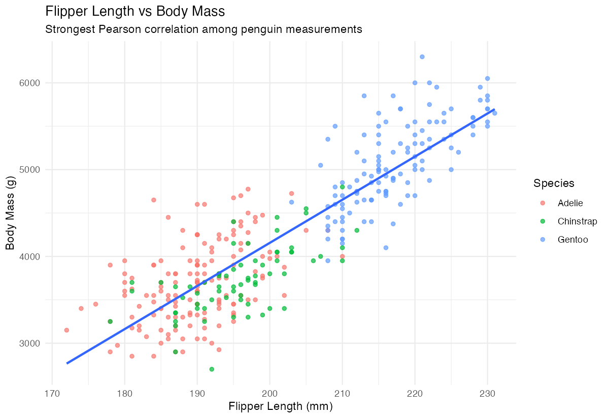
The scatter plot confirms the strong positive relationship between flipper length and body mass across all species.
Summary
- Use
cor()withmethod = "pearson"to compute correlation matrices for multiple variables - The
use = "complete.obs"parameter handles missing values by excluding incomplete cases - Group-wise correlations reveal how relationships vary across different categories or species
- Correlation values range from -1 (perfect negative) to 1 (perfect positive), with 0 indicating no linear relationship
Always visualize strong correlations to confirm the relationship pattern and identify potential outliers