Learn how to compute Pearson, Spearman, and Kendall correlation in R using the cor() function with practical examples.
Published
August 17, 2022
In this tutorial, we will learn how to compute correlation between two numerical variables in R using the cor() function. We’ll cover three correlation methods:
Pearson - measures linear relationship (default)
Spearman - measures monotonic relationship using ranks
Kendall - measures ordinal association
Correlation values range from -1 to +1: - -1: Perfect negative correlation - 0: No correlation - +1: Perfect positive correlation
Spearman correlation measures monotonic relationships using ranks. It’s more robust to outliers and works well for non-linear but monotonic relationships.
You can also compute correlation between standalone vectors:
set.seed(42)# Generate correlated datax <-rnorm(100, mean =50, sd =10)y <- x *2+rnorm(100, mean =0, sd =5) # y is related to x# Compute correlationscor(x, y, method ="pearson")cor(x, y, method ="spearman")
Correlation Matrix
To compute correlations between multiple variables at once:
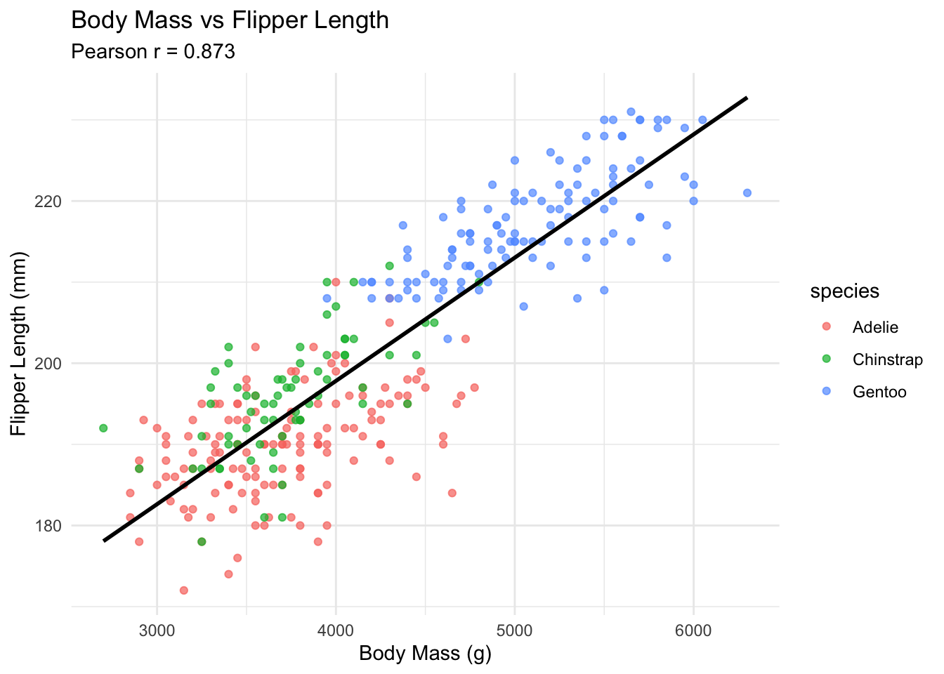
---title: "Computing Correlation with R"date: 2022-08-17categories: ['statistics', 'correlation']description: "Learn how to compute Pearson, Spearman, and Kendall correlation in R using the cor() function with practical examples."format: html: code-fold: false code-tools: true---In this tutorial, we will learn how to compute correlation between two numerical variables in R using the [`cor()`](/statistics/how-to-pearson-correlation-in-r.html) function. We'll cover three correlation methods:- **Pearson** - measures linear relationship (default)- **Spearman** - measures monotonic relationship using ranks- **Kendall** - measures ordinal associationCorrelation values range from -1 to +1:- **-1**: Perfect negative correlation- **0**: No correlation- **+1**: Perfect positive correlation## Setup```{r}#| message: falselibrary(palmerpenguins)library(tidyverse)df <- penguins %>%drop_na()head(df)```## Pearson Correlation (Default)Pearson correlation measures the **linear relationship** between two variables. It's the default method in `cor()`.```r# Correlation between body mass and flipper lengthcor(df$body_mass_g, df$flipper_length_mm)```This shows a strong positive correlation (~0.87) - penguins with larger body mass tend to have longer flippers.```r# Explicitly specify methodcor(df$body_mass_g, df$flipper_length_mm, method ="pearson")```## Spearman CorrelationSpearman correlation measures **monotonic relationships** using ranks. It's more robust to outliers and works well for non-linear but monotonic relationships.```rcor(df$body_mass_g, df$flipper_length_mm, method ="spearman")```## Kendall CorrelationKendall's tau measures **ordinal association** between variables. It's often more robust than Spearman for small samples.```rcor(df$body_mass_g, df$flipper_length_mm, method ="kendall")```## Comparing All Three Methods```r# Create a comparisonmethods <-c("pearson", "spearman", "kendall")correlations <-sapply(methods, function(m) {cor(df$body_mass_g, df$flipper_length_mm, method = m)})data.frame(Method = methods,Correlation =round(correlations, 4))```## Correlation with VectorsYou can also compute correlation between standalone vectors:```rset.seed(42)# Generate correlated datax <-rnorm(100, mean =50, sd =10)y <- x *2+rnorm(100, mean =0, sd =5) # y is related to x# Compute correlationscor(x, y, method ="pearson")cor(x, y, method ="spearman")```## Correlation MatrixTo compute correlations between multiple variables at once:```r# Select numeric columnsnumeric_cols <- df %>%select(bill_length_mm, bill_depth_mm, flipper_length_mm, body_mass_g)# Correlation matrix with Pearsonround(cor(numeric_cols), 2)``````r# Correlation matrix with Spearmanround(cor(numeric_cols, method ="spearman"), 2)```## Visualizing Correlation```{r}#| label: fig-correlation#| fig-cap: "Scatter plot showing correlation between body mass and flipper length"ggplot(df, aes(x = body_mass_g, y = flipper_length_mm)) +geom_point(aes(color = species), alpha =0.7) +geom_smooth(method ="lm", se =FALSE, color ="black") +labs(title ="Body Mass vs Flipper Length",subtitle =paste("Pearson r =", round(cor(df$body_mass_g, df$flipper_length_mm), 3)),x ="Body Mass (g)",y ="Flipper Length (mm)" ) +theme_minimal()```## When to Use Each Method| Method | Use When ||--------|----------|| **Pearson** | Data is normally distributed, relationship is linear || **Spearman** | Data has outliers, relationship is monotonic but not linear || **Kendall** | Small sample size, ordinal data, more robust estimation needed |## Summary- Use `cor(x, y)` for Pearson correlation (default)- Use `cor(x, y, method = "spearman")` for rank-based correlation- Use `cor(x, y, method = "kendall")` for ordinal association- All methods return values from -1 to +1## Related Tutorials- [How to correlation matrix in R](how-to-correlation-matrix-in-r.html)- [Understanding the Normal Distribution in R](understanding-normal-distribution.html)- [How to extract residuals from a linear regression model](extract-residuals-from-a-linear-regression-model.html)- [How to Compute Z-Score of Multiple Columns](compute-z-score-of-multiple-columns.html)- [How to get p-value from linear regression model](get-p-value-from-linear-regression-model.html)