How to ANOVA two-way in R
Introduction
Two-way ANOVA tests whether two categorical variables (factors) have significant effects on a continuous outcome variable, including their interaction. Use this when you want to examine how two different grouping variables simultaneously influence your response variable.
Getting Started
library(tidyverse)
library(palmerpenguins)
Example 1: Basic Usage
The Problem
We want to test if penguin body mass differs by both species and sex, and whether there’s an interaction between these factors.
Step 1: Explore the Data
First, let’s examine our variables and check for missing values.
penguins |>
  select(body_mass_g, species, sex) |>
  summary()

# Remove missing values
penguins_clean <- penguins |>
  filter(!is.na(body_mass_g), !is.na(sex))
We now have a clean dataset with 333 penguins across 3 species and 2 sexes.
Step 2: Visualize the Data
Create a plot to visualize potential differences between groups.
penguins_clean |>
  ggplot(aes(x = species, y = body_mass_g, fill = sex)) +
  geom_boxplot(alpha = 0.85) +
  labs(title = "Penguin Body Mass by Species and Sex",
       x = "Species", y = "Body Mass (g)")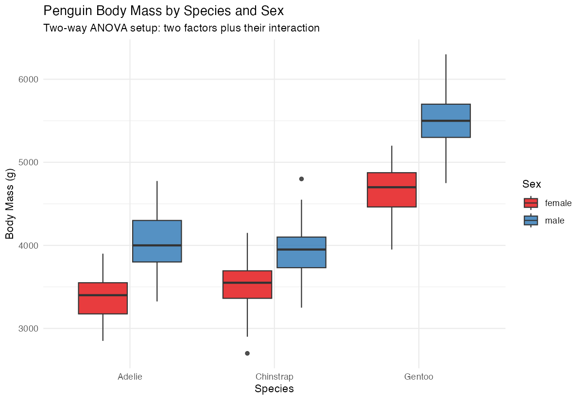
The plot suggests both species and sex affect body mass, with possible interactions.
Step 3: Run Two-Way ANOVA
Perform the ANOVA test including the interaction term.
# Fit the two-way ANOVA model
anova_model <- aov(body_mass_g ~ species * sex, data = penguins_clean)

# View results
summary(anova_model)
The results show significant main effects for both species and sex, plus a significant interaction.
Step 4: Check Model Assumptions
Verify that our data meets ANOVA assumptions.
# Check residuals
par(mfrow = c(2, 2))
plot(anova_model)
par(mfrow = c(1, 1))
The diagnostic plots show our assumptions are reasonably met with normal residuals and equal variances.
Example 2: Practical Application
The Problem
A researcher wants to determine if car fuel efficiency (mpg) is affected by both transmission type (automatic vs manual) and number of cylinders. They also want to know if these factors interact with each other.
Step 1: Prepare the Data
Convert variables to appropriate types and explore the structure.
# Prepare mtcars data
mtcars_clean <- mtcars |>
  mutate(
    transmission = factor(am, labels = c("automatic", "manual")),
    cylinders = factor(cyl)
  )

head(mtcars_clean[c("mpg", "transmission", "cylinders")])
We’ve converted transmission and cylinders to factors for proper ANOVA analysis.
Step 2: Explore Group Means
Calculate descriptive statistics for each combination of factors.
mtcars_clean |>
  group_by(transmission, cylinders) |>
  summarise(
    mean_mpg = mean(mpg),
    sd_mpg = sd(mpg),
    n = n(),
    .groups = "drop"
  )
Manual transmissions generally show higher mpg, and fewer cylinders associate with better fuel efficiency.
Step 3: Visualize the Interaction
Create a plot to examine potential interactions between factors.
mtcars_clean |>
  ggplot(aes(x = cylinders, y = mpg, color = transmission)) +
  geom_point(size = 3, alpha = 0.7,
             position = position_jitter(width = 0.1, height = 0)) +
  stat_summary(fun = mean, geom = "line",
               aes(group = transmission), linewidth = 1.2) +
  labs(title = "MPG by Cylinders and Transmission Type",
       x = "Number of Cylinders", y = "Miles per Gallon")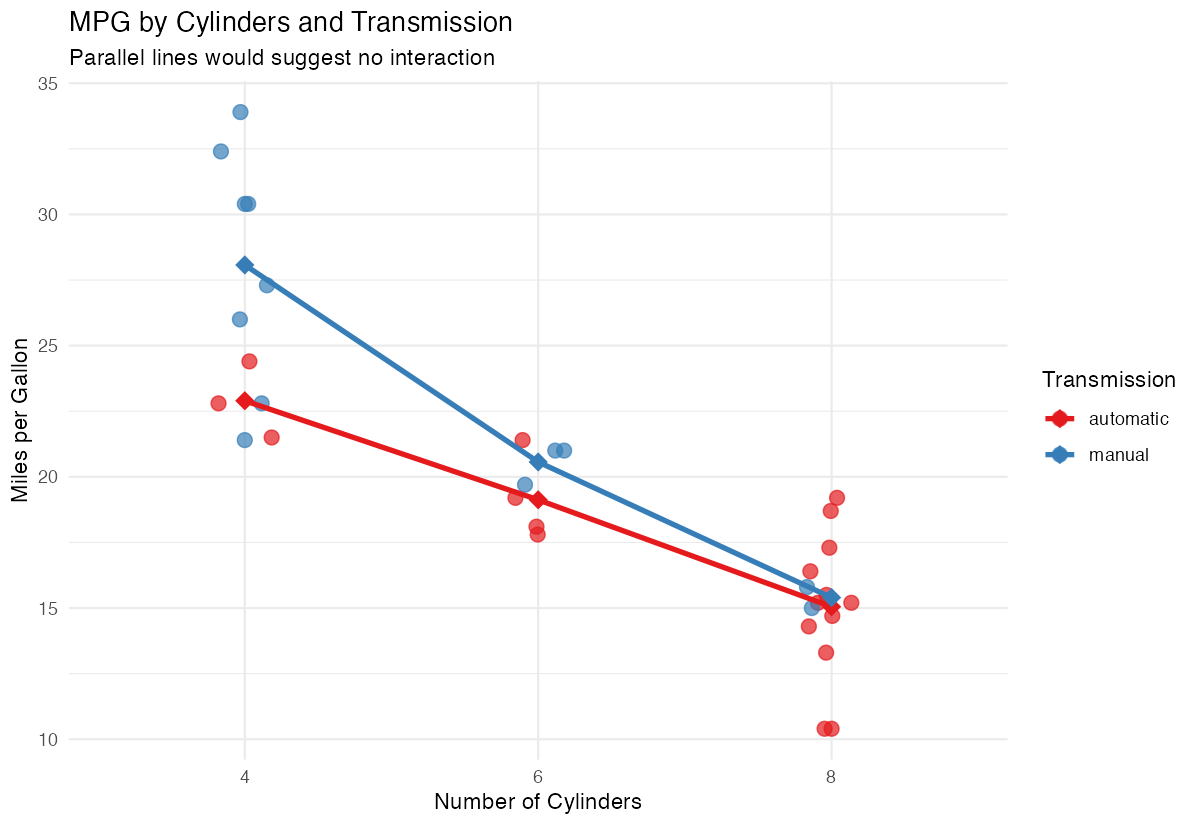
The plot suggests transmission effects may vary across cylinder groups.
Step 4: Conduct Two-Way ANOVA
Run the complete analysis including interaction effects.
# Fit the model
car_anova <- aov(mpg ~ transmission * cylinders, data = mtcars_clean)

# Display results
summary(car_anova)
Results show significant main effects for cylinders but not transmission, with no significant interaction.
Step 5: Post-Hoc Analysis
Since cylinders has multiple levels, perform pairwise comparisons.
# Tukey's HSD for multiple comparisons
TukeyHSD(car_anova, "cylinders")
The post-hoc test reveals which specific cylinder groups differ significantly from each other.
Summary
- Two-way ANOVA examines effects of two categorical variables on a continuous outcome
- Include interaction terms using
*to test if factor effects depend on each other
- Always check model assumptions using diagnostic plots before interpreting results
- Use post-hoc tests like TukeyHSD for factors with more than two levels
Visualize your data first to understand potential patterns and interactions