How to Perform One-Way ANOVA in R
Introduction
One-way ANOVA (Analysis of Variance) tests whether the means of three or more groups are significantly different from each other. Use this test when you have one categorical predictor variable and one continuous outcome variable, and you want to compare group means.
When to use one-way ANOVA: - Comparing means across 3+ independent groups - Testing if a categorical factor affects a continuous outcome - Analyzing experimental designs with one treatment factor - Extending the two-sample t-test to multiple groups
The Math Behind ANOVA
ANOVA partitions total variance into between-group and within-group components:
F = (Between-group variance) / (Within-group variance)
   = (SSB / dfB) / (SSW / dfW)
   = MSB / MSW
Where: - SSB (Sum of Squares Between) = Σnᵢ(x̄ᵢ - x̄)² — how much group means differ from overall mean - SSW (Sum of Squares Within) = ΣΣ(xᵢⱼ - x̄ᵢ)² — how much observations vary within groups - dfB = k - 1 (k = number of groups) - dfW = N - k (N = total observations)
A large F-ratio indicates group means differ more than expected from random variation within groups.
Getting Started
library(tidyverse)
library(palmerpenguins)
Example 1: Basic Usage
The Problem
We want to test if penguin body mass differs significantly across the three species (Adelie, Chinstrap, and Gentoo). This is a classic one-way ANOVA scenario with species as our grouping variable.
Step 1: Explore the Data
First, let’s examine our data structure and get basic statistics for each group.
# View the data structure
penguins |>
  select(species, body_mass_g) |>
  glimpse()
This shows us we have a factor variable (species) and a numeric variable (body_mass_g) - perfect for ANOVA.
Step 2: Calculate Group Statistics
Let’s calculate summary statistics to understand differences between groups.
# Get descriptive statistics by species
summary_stats <- penguins |>
  group_by(species) |>
  summarise(
    count = n(),
    mean_mass = mean(body_mass_g, na.rm = TRUE),
    sd_mass = sd(body_mass_g, na.rm = TRUE)
  )
print(summary_stats)
The output shows different sample sizes and mean body masses across species, suggesting potential differences.
Step 3: Visualize Group Differences
Create a boxplot to visually assess differences between groups.
# Create boxplot to visualize differences
penguins |>
  filter(!is.na(body_mass_g)) |>
  ggplot(aes(x = species, y = body_mass_g, fill = species)) +
  geom_boxplot(alpha = 0.8) +
  labs(title = "Penguin Body Mass by Species",
       x = "Species", y = "Body Mass (g)") +
  theme(legend.position = "none")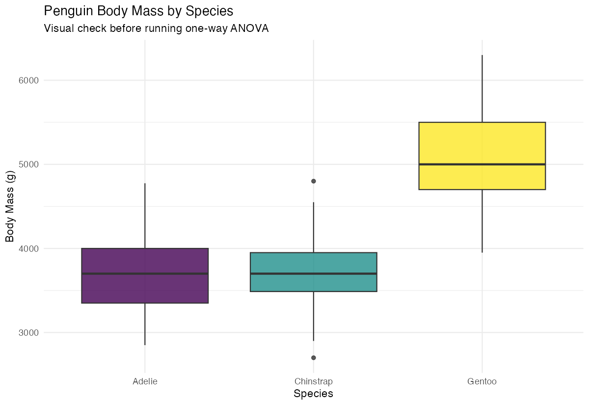
The boxplot reveals clear visual differences in body mass distributions across the three species.
Step 4: Perform One-Way ANOVA
Now we’ll conduct the actual ANOVA test using the aov() function.
# Run one-way ANOVA
anova_result <- aov(body_mass_g ~ species, data = penguins)
summary(anova_result)
The ANOVA output shows an F-statistic and p-value to determine if group means differ significantly.
Example 2: Practical Application
The Problem
A car manufacturer wants to determine if fuel efficiency (mpg) differs significantly between cars with different numbers of cylinders. We’ll use the mtcars dataset to analyze whether 4-cylinder, 6-cylinder, and 8-cylinder cars have different average fuel efficiency.
Step 1: Prepare the Data
We need to convert the cylinder variable to a factor and examine our data.
# Prepare data and convert cyl to factor
mtcars_clean <- mtcars |>
  mutate(cyl_factor = as.factor(cyl)) |>
  select(mpg, cyl_factor)

# Check the data
head(mtcars_clean)
Converting cylinders to a factor ensures R treats it as a categorical grouping variable rather than numeric.
Step 2: Check Assumptions
ANOVA assumes normal distribution within groups and equal variances.
# Check normality with Q-Q plots by group
mtcars_clean |>
  ggplot(aes(sample = mpg)) +
  stat_qq() + stat_qq_line() +
  facet_wrap(~cyl_factor) +
  labs(title = "Q-Q Plots by Cylinder Group")
The Q-Q plots help us assess whether the data within each group follows a normal distribution.
Step 3: Perform ANOVA with Post-hoc Tests
Run the ANOVA and follow up with pairwise comparisons.
# Run ANOVA
car_anova <- aov(mpg ~ cyl_factor, data = mtcars_clean)
summary(car_anova)

# Perform Tukey's HSD for pairwise comparisons
TukeyHSD(car_anova)
Tukey’s HSD test tells us which specific pairs of groups differ significantly from each other.
Step 4: Interpret and Visualize Results
Create a comprehensive visualization of the results.
# Create detailed boxplot with mean points
mtcars_clean |>
  ggplot(aes(x = cyl_factor, y = mpg, fill = cyl_factor)) +
  geom_boxplot(alpha = 0.7) +
  stat_summary(fun = mean, geom = "point",
               color = "red", size = 3) +
  labs(title = "Fuel Efficiency by Cylinder Count",
       x = "Number of Cylinders", y = "Miles per Gallon") +
  theme(legend.position = "none")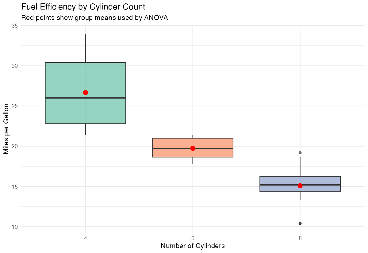
This visualization combines boxplots with mean points to clearly show both distributions and central tendencies.
Assumptions and Limitations
Key assumptions of one-way ANOVA:
- Independence: Observations are independent within and across groups
- Normality: Data within each group should be approximately normally distributed
- Homogeneity of variance: Variance should be similar across all groups
Test for equal variances (Levene’s test):
library(car)
leveneTest(body_mass_g ~ species, data = penguins)
If p < 0.05, variances are significantly different. Use Welch’s ANOVA instead:
# Welch's ANOVA - doesn't assume equal variances
oneway.test(body_mass_g ~ species, data = penguins, var.equal = FALSE)
Test for normality (Shapiro-Wilk test by group):
penguins |>
  group_by(species) |>
  summarise(
    shapiro_p = shapiro.test(body_mass_g)$p.value
  )
When assumptions are violated:
- Non-normality: ANOVA is robust with large samples (n > 30 per group). Otherwise, use Kruskal-Wallis test
- Unequal variances: Use Welch’s ANOVA via
oneway.test(var.equal = FALSE) - Non-independence: Use repeated measures ANOVA or mixed models
# Non-parametric alternative (Kruskal-Wallis)
kruskal.test(body_mass_g ~ species, data = penguins)
Common Mistakes
1. Not doing post-hoc tests after significant ANOVA
ANOVA tells you groups differ, but not which ones. Always follow up:
# Tukey's HSD for pairwise comparisons
TukeyHSD(anova_result)

# Or pairwise t-tests with correction
pairwise.t.test(penguins$body_mass_g, penguins$species, p.adjust.method = "bonferroni")
2. Using multiple t-tests instead of ANOVA
Running many t-tests inflates Type I error. With 3 groups, you’d do 3 comparisons, making the family-wise error rate ~14% instead of 5%.
3. Ignoring the homogeneity of variance assumption
# Check variance ratios
penguins |>
  group_by(species) |>
  summarise(variance = var(body_mass_g, na.rm = TRUE))
If the largest variance is more than 4× the smallest, consider Welch’s ANOVA.
4. Not reporting effect size
Statistical significance doesn’t indicate practical importance. Report eta-squared (η²):
# Calculate eta-squared
ss_between <- sum(anova_result$residuals^2)
ss_total <- var(penguins$body_mass_g, na.rm = TRUE) * (nrow(na.omit(penguins)) - 1)
eta_squared <- 1 - (ss_between / ss_total)

# Or use effectsize package
library(effectsize)
eta_squared(anova_result)- Small: η² = 0.01
- Medium: η² = 0.06
- Large: η² = 0.14
Summary
- One-way ANOVA compares means across three or more independent groups using the
aov()function - Always explore your data first with summary statistics and visualizations before running the test
- Check ANOVA assumptions: normality within groups and equal variances across groups
- Use
TukeyHSD()for post-hoc pairwise comparisons when ANOVA is significant - Report effect size (eta-squared) alongside p-values