How to Perform Logistic Regression in R
Introduction
Logistic regression is a statistical method used to predict binary outcomes (yes/no, success/failure, 0/1) based on one or more predictor variables. Unlike linear regression which predicts continuous values, logistic regression uses the logistic function to model the probability that an instance belongs to a particular category.
You would use logistic regression when your dependent variable is categorical with two levels, such as predicting whether an email is spam, if a customer will purchase a product, or whether a medical treatment will be successful. It’s particularly valuable because it provides both predictions and probabilities, along with interpretable coefficients that show how each predictor affects the odds of the outcome.
The Math Behind Logistic Regression
Logistic regression models the probability of the outcome using the logistic (sigmoid) function:
P(Y=1) = 1 / (1 + e^(-z))Where z is the linear combination of predictors:
z = β₀ + β₁X₁ + β₂X₂ + ... + βₙXₙThe key insight is that we’re modeling the log-odds (also called logit):
log(P / (1-P)) = β₀ + β₁X₁ + β₂X₂ + ...This means: - Each coefficient βᵢ represents the change in log-odds for a one-unit increase in Xᵢ - To get odds ratios, exponentiate the coefficients: exp(βᵢ) - An odds ratio of 2 means the odds double for each unit increase in the predictor
Getting Started
library(tidyverse)
library(palmerpenguins)
Example 1: Basic Usage
The Problem
We want to predict penguin sex (male/female) based on body mass. This is a binary classification problem - perfect for logistic regression.
Preparing the data
First, load the data and remove rows with missing values in our variables of interest:
data(penguins)

penguins_clean <- penguins |>
  filter(!is.na(sex), !is.na(body_mass_g))
Fitting the model
Use glm() with family = binomial to fit a logistic regression:
model_basic <- glm(sex ~ body_mass_g,
                   data = penguins_clean,
                   family = binomial)

summary(model_basic)
The family = binomial argument tells R we want logistic regression (not linear regression).
Making predictions
Use predict() with type = "response" to get probabilities (not log-odds):
penguins_clean <- penguins_clean |>
  mutate(
    predicted_prob = predict(model_basic, type = "response"),
    predicted_sex = ifelse(predicted_prob > 0.5, "male", "female")
  )
Probabilities > 0.5 are classified as “male”, otherwise “female”.
Checking accuracy
accuracy <- mean(penguins_clean$sex == penguins_clean$predicted_sex)
print(paste("Accuracy:", round(accuracy, 3)))
This tells us what percentage of predictions were correct.
Example 2: Practical Application
The Problem
A single predictor (body mass) might not be enough. Let’s build a better model using multiple measurements: bill length, bill depth, flipper length, body mass, and species.
Preparing the data
Remove rows with missing values in any of our predictors:
penguins_full <- penguins |>
  filter(
    !is.na(sex),
    !is.na(bill_length_mm),
    !is.na(bill_depth_mm),
    !is.na(flipper_length_mm),
    !is.na(body_mass_g)
  )
Fitting the multiple logistic regression
Add multiple predictors separated by +:
model_full <- glm(
  sex ~ bill_length_mm + bill_depth_mm + flipper_length_mm + body_mass_g + species,
  data = penguins_full,
  family = binomial
)

summary(model_full)
The summary shows coefficients for each predictor. Positive coefficients increase the probability of “male”, negative coefficients decrease it.
Making predictions and evaluating
penguins_results <- penguins_full |>
  mutate(
    predicted_prob = predict(model_full, type = "response"),
    predicted_sex = ifelse(predicted_prob > 0.5, "male", "female"),
    correct_prediction = sex == predicted_sex
  )
Calculating accuracy
accuracy_full <- mean(penguins_results$correct_prediction)
print(paste("Full model accuracy:", round(accuracy_full, 3)))
The multi-predictor model should have higher accuracy than the single-predictor model.
Creating a confusion matrix
A confusion matrix shows how many predictions were correct vs incorrect for each class:
confusion_matrix <- penguins_results |>
  count(sex, predicted_sex) |>
  pivot_wider(names_from = predicted_sex, values_from = n, values_fill = 0)

print(confusion_matrix)
This shows true positives, true negatives, false positives, and false negatives.
Visualizing predicted probabilities
penguins_results |>
  ggplot(aes(x = predicted_prob, fill = sex)) +
  geom_histogram(alpha = 0.7, bins = 20, position = "identity") +
  labs(
    title = "Distribution of Predicted Probabilities by Actual Sex",
    x = "Predicted Probability of Being Male",
    y = "Count"
  ) +
  theme_minimal()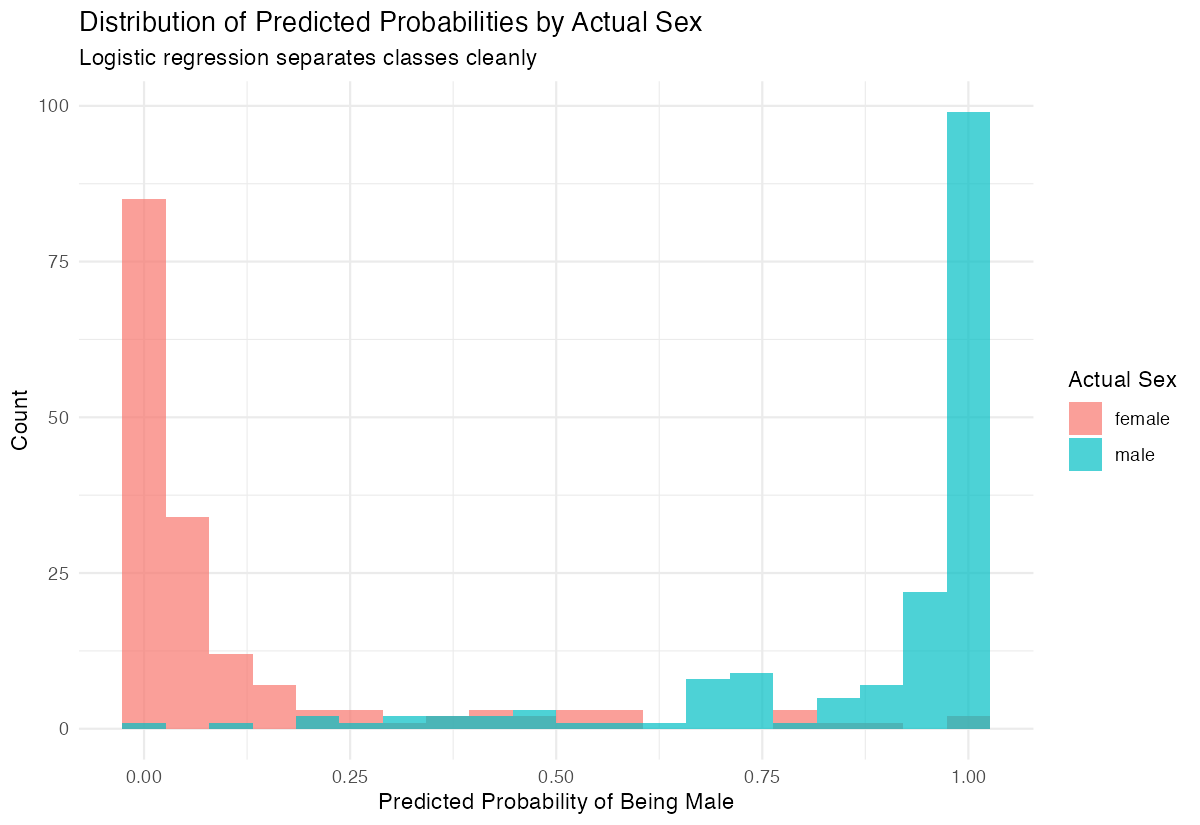
A good model shows clear separation: actual males should have high predicted probabilities, females should have low ones.
Interpreting Odds Ratios
To understand coefficient magnitudes, calculate odds ratios:
# Get odds ratios from model coefficients
odds_ratios <- exp(coef(model_full))
print(round(odds_ratios, 3))
Interpretation example: If the odds ratio for body_mass_g is 1.005, it means for each additional gram of body mass, the odds of being male increase by 0.5%. For a 100g increase, odds increase by approximately 65% (1.005^100 ≈ 1.65).
Assumptions and Limitations
Key assumptions of logistic regression:
- Binary outcome: The dependent variable must have exactly two categories
- Independence: Observations should be independent of each other
- No multicollinearity: Predictors should not be highly correlated with each other
- Linear relationship: The log-odds should be linearly related to continuous predictors
- Large sample size: General rule is at least 10-20 events per predictor variable
Check for multicollinearity:
# Check variance inflation factors
library(car)
vif(model_full)
VIF values above 5-10 indicate problematic multicollinearity.
Don’t use logistic regression when:
- Your outcome has more than 2 categories (use multinomial logistic regression instead)
- You have very few events relative to predictors (causes separation problems)
- Relationships between predictors and log-odds are highly non-linear
Common Mistakes
1. Forgetting family = binomial
# Wrong - fits linear regression
model_wrong <- glm(sex ~ body_mass_g, data = penguins_clean)

# Correct - fits logistic regression
model_right <- glm(sex ~ body_mass_g, data = penguins_clean, family = binomial)
2. Using predictions without type = "response"
# Wrong - returns log-odds (hard to interpret)
predict(model_basic)

# Correct - returns probabilities (0 to 1)
predict(model_basic, type = "response")
3. Interpreting coefficients as probabilities
Coefficients are in log-odds scale, not probability scale. A coefficient of 0.5 doesn’t mean “50% increase in probability” - it means the log-odds increase by 0.5.
4. Ignoring class imbalance
If one class is much more common, the model may predict only the majority class. Consider: - Adjusting the classification threshold - Using stratified sampling - Using metrics like AUC-ROC instead of accuracy
Summary
- Use
glm(y ~ x, family = binomial)for logistic regression - Use
predict(model, type = "response")to get probabilities (0-1), not log-odds - Classify using a threshold:
ifelse(prob > 0.5, "positive", "negative") - Multiple predictors usually improve accuracy
- Evaluate with accuracy and confusion matrix
Visualize predicted probabilities to assess model quality