How to Create a Correlation Matrix in R
1. Introduction
A correlation matrix is a table showing correlation coefficients between multiple variables. Each cell in the matrix represents the correlation between two variables, with values ranging from -1 to +1. A correlation of +1 indicates perfect positive correlation, -1 indicates perfect negative correlation, and 0 indicates no linear relationship.
Correlation matrices are invaluable when exploring relationships in datasets with multiple numeric variables. You’d use one when conducting exploratory data analysis, identifying multicollinearity before regression modeling, or understanding which variables move together in your data. They’re particularly useful in fields like finance (asset correlations), psychology (trait relationships), and biology (morphological measurements).
The primary assumption is that relationships between variables are linear. Correlation matrices work best with continuous numeric data that follows roughly normal distributions. They measure linear associations only - strong non-linear relationships might show weak correlations. Additionally, correlation doesn’t imply causation, and outliers can heavily influence results.
2. The Math
The correlation coefficient (Pearson’s r) between two variables X and Y is calculated as:
r = Σ[(Xi - X̄)(Yi - Ȳ)] / √[Σ(Xi - X̄)² × Σ(Yi - Ȳ)²]Where: - Xi, Yi are individual data points - X̄, Ȳ are the means of X and Y - Σ means “sum of”
This formula measures how much the variables vary together (numerator) relative to how much they vary separately (denominator). The result is standardized between -1 and +1.
For a correlation matrix, this calculation is performed for every pair of variables in your dataset, creating a symmetric matrix where the diagonal always equals 1 (each variable perfectly correlates with itself).
3. R Implementation
Let’s explore correlation matrices using the Palmer Penguins dataset:
library(tidyverse)
library(palmerpenguins)
library(corrplot)

# Load and examine the data
data(penguins)
glimpse(penguins)
Rows: 344
Columns: 8
$ species <fct> Adelie, Adelie, Adelie, Adelie, Adelie, Adelie, A...
$ island <fct> Torgersen, Torgersen, Torgersen, Torgersen, Torge...
$ bill_length_mm <dbl> 39.1, 39.5, 40.3, NA, 36.7, 39.3, 38.9, 39.2, 34...
$ bill_depth_mm <dbl> 18.7, 17.4, 18.0, NA, 19.3, 20.6, 17.8, 19.6, 18...
$ flipper_length_mm <int> 181, 186, 195, NA, 193, 190, 181, 195, 193, 190, ...
$ body_mass_g <int> 3750, 3800, 3250, NA, 3450, 3650, 3625, 4675, 380...
$ sex <fct> male, female, female, NA, female, male, female, ma...
$ year <int> 2007, 2007, 2007, 2007, 2007, 2007, 2007, 2007, 2...# Create correlation matrix using base R
numeric_vars <- penguins %>%
select(bill_length_mm, bill_depth_mm, flipper_length_mm, body_mass_g) %>%
na.omit()
# Base R correlation matrix
cor_matrix <- cor(numeric_vars)
print(cor_matrix) bill_length_mm bill_depth_mm flipper_length_mm body_mass_g
bill_length_mm 1.0000000 -0.2286256 0.6561813 0.5951098
bill_depth_mm -0.2286256 1.0000000 -0.5838512 -0.4719156
flipper_length_mm 0.6561813 -0.5838512 1.0000000 0.8712018
body_mass_g 0.5951098 -0.4719156 0.8712018 1.00000004. Full Worked Example
Let’s conduct a complete correlation analysis of penguin morphological measurements:
# Step 1: Prepare the data
penguin_numeric <- penguins %>%
  select(bill_length_mm, bill_depth_mm, flipper_length_mm, body_mass_g) %>%
  na.omit()

# Step 2: Calculate correlation matrix with significance tests
cor_result <- cor.test(penguin_numeric$bill_length_mm, penguin_numeric$flipper_length_mm)
print(cor_result)
Pearson's product-moment correlation
data: penguin_numeric$bill_length_mm and penguin_numeric$flipper_length_mm
t = 15.73, df = 340, p-value < 2.2e-16
alternative hypothesis: true correlation is not equal to 0
95 percent confidence interval:
0.5993967 0.7065473
sample estimates:
cor
0.6561813# Step 3: Create complete correlation matrix
correlation_matrix <- cor(penguin_numeric)
round(correlation_matrix, 3) bill_length_mm bill_depth_mm flipper_length_mm body_mass_g
bill_length_mm 1.000 -0.229 0.656 0.595
bill_depth_mm -0.229 1.000 -0.584 -0.472
flipper_length_mm 0.656 -0.584 1.000 0.871
body_mass_g 0.595 -0.472 0.871 1.000Interpretation: - Strongest positive correlation: Flipper length and body mass (r = 0.871) - larger penguins have longer flippers - Strongest negative correlation: Flipper length and bill depth (r = -0.584) - penguins with longer flippers tend to have shallower bills - Moderate positive correlation: Bill length and flipper length (r = 0.656) - longer bills associate with longer flippers - Weak negative correlation: Bill length and bill depth (r = -0.229) - slight tendency for longer bills to be shallower
5. Visualization
# Create a correlation plot
library(corrplot)

corrplot(correlation_matrix,
         method = "color",
         type = "upper",
         addCoef.col = "black",
         tl.col = "black",
         tl.srt = 45,
         diag = FALSE,
         title = "Penguin Morphological Correlations",
         mar = c(0,0,2,0))
# Alternative ggplot2 heatmap
library(reshape2)
cor_melted <- melt(correlation_matrix)
ggplot(cor_melted, aes(Var1, Var2, fill = value)) +
geom_tile() +
geom_text(aes(label = round(value, 2)), color = "white", size = 4) +
scale_fill_gradient2(low = "blue", mid = "white", high = "red",
midpoint = 0, limit = c(-1,1)) +
theme_minimal() +
theme(axis.text.x = element_text(angle = 45, hjust = 1)) +
labs(title = "Penguin Correlation Matrix Heatmap",
x = "", y = "", fill = "Correlation")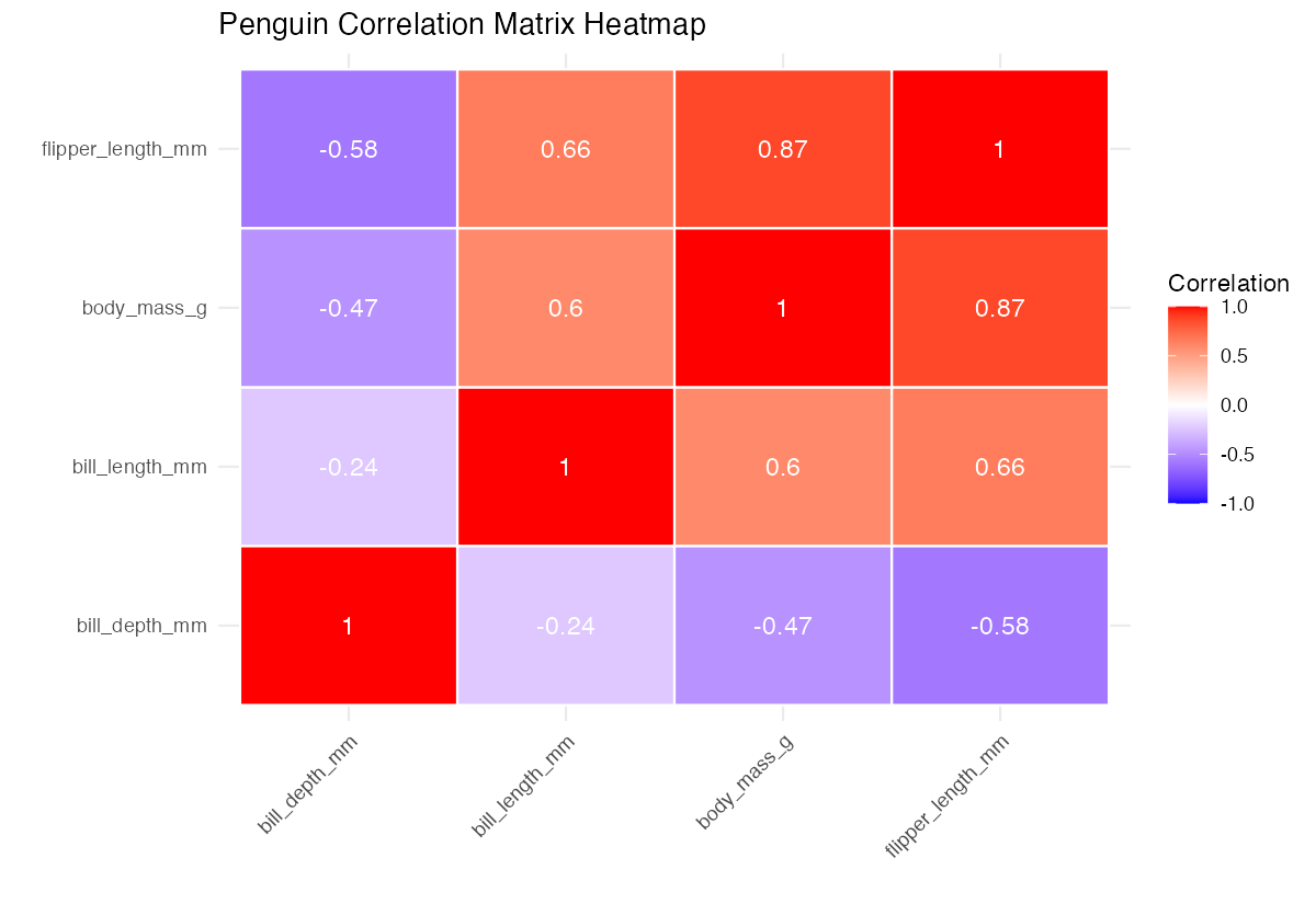
This visualization shows correlation strength through color intensity and displays exact values. Blue indicates negative correlations, red shows positive correlations, and white represents no correlation. The plot reveals clear patterns: body size measurements (flipper length, body mass) cluster together with strong positive correlations, while bill depth shows negative relationships with most other measurements.
6. Assumptions & Limitations
Don’t use correlation matrices when: - Data is not numeric: Categorical variables need different association measures (Cramér’s V, phi coefficient) - Relationships are non-linear: Consider Spearman correlation or transformation first - Severe outliers present: They can create misleading correlations - Data is heavily skewed: May need log transformation or robust correlation methods
Common violations and solutions:
# Check for outliers
penguin_numeric %>%
  pivot_longer(everything()) %>%
  ggplot(aes(x = name, y = value)) +
  geom_boxplot() +
  facet_wrap(~name, scales = "free")

# Spearman correlation for non-linear relationships
cor(penguin_numeric, method = "spearman")
Correlation matrices assume linear relationships and can miss important non-linear patterns. They’re also sensitive to sample size - small samples produce unreliable estimates, while very large samples make tiny correlations appear statistically significant but practically meaningless.
7. Common Mistakes
1. Confusing correlation with causation
# Wrong interpretation: "Body mass causes flipper length"
# Correct: "Body mass and flipper length are strongly associated"
cor.test(penguin_numeric$body_mass_g, penguin_numeric$flipper_length_mm)
2. Ignoring missing data patterns
# Bad: Excluding rows with ANY missing values
penguins %>% select(bill_length_mm:body_mass_g) %>% na.omit()

# Better: Check missing data patterns first
library(VIM)
aggr(penguins, col = c('navyblue','red'), numbers = TRUE)
3. Over-interpreting weak correlations in large samples Small correlations (|r| < 0.3) might be statistically significant but practically meaningless. Always consider effect size alongside p-values, and focus on correlations with practical significance for your domain.