---
title: "Introduction to Mixed Effects Models in R"
description: "Learn the basics of mixed effects models in R using the sleepstudy dataset. Understand when and why to use them for longitudinal data, with step-by-step examples using lme4."
date: 2026-02-22
categories: ["statistics", "mixed effects models"]
format:
html:
code-fold: false
code-tools: true
---
## Introduction
Mixed effects models (also called multilevel models or hierarchical models) are essential when your data has **repeated measurements** from the same subjects. For example:
- Reaction times measured daily during a sleep study
- Patient health scores tracked over multiple visits
- Student test scores across semesters
- Plant growth measured weekly
[Regular regression](/statistics/how-to-linear-regression-basics-in-r.html) assumes all observations are independent. But when you measure the same person multiple times, those measurements are correlated - they share that person's baseline characteristics. Ignoring this leads to incorrect conclusions.
## The Sleep Study Dataset
The `sleepstudy` dataset from the [`lme4`](https://cran.r-project.org/package=lme4) package is a classic example of longitudinal data. Researchers measured **reaction times** of **18 subjects** over **10 days** of sleep deprivation. The data comes from a study by Gregory Belenky and colleagues on the effects of sleep deprivation on cognitive performance.
```{r}
#| message: false
#| warning: false
# Load required packages
library(tidyverse)   # https://www.tidyverse.org/
library(lme4)        # https://cran.r-project.org/package=lme4
library(broom.mixed) # https://cran.r-project.org/package=broom.mixed

# Look at the data
head(sleepstudy, 12)
```
The data structure:
- **Reaction**: Response time in milliseconds (outcome variable)
- **Days**: Days of sleep deprivation (0-9)
- **Subject**: Subject identifier (18 subjects)
```{r}
# Check the structure
sleepstudy |>
  group_by(Subject) |>
  summarise(
    n_measurements = n(),
    first_day = min(Days),
    last_day = max(Days)
  ) |>
  head()
```
Each subject has 10 measurements - one per day. This is **longitudinal data**: the same people measured repeatedly over time.
### Dataset Summary
| Variable | Type | Description | Values |
|----------|------|-------------|--------|
| **Reaction** | Numeric (outcome) | Response time in milliseconds | 194 - 466 ms |
| **Days** | Numeric (predictor) | Days of sleep deprivation | 0, 1, 2, ... 9 |
| **Subject** | Factor (grouping) | Unique subject identifier | 18 subjects |
### Repeated Measures Structure
| Level | Count | Description |
|-------|-------|-------------|
| **Subjects** | 18 | Independent individuals in the study |
| **Measurements per subject** | 10 | One measurement per day (Days 0-9) |
| **Total observations** | 180 | 18 subjects × 10 days |
::: {.callout-important}
## Key Insight: Rows ≠ Independent Observations
We have **180 rows** but only **18 independent units**. Regular regression would treat this as 180 independent observations - that's wrong! The 10 measurements from Subject 308 are more similar to each other than to measurements from Subject 309.
:::
## Why Mixed Effects Models?
### The Problem: Individual Differences
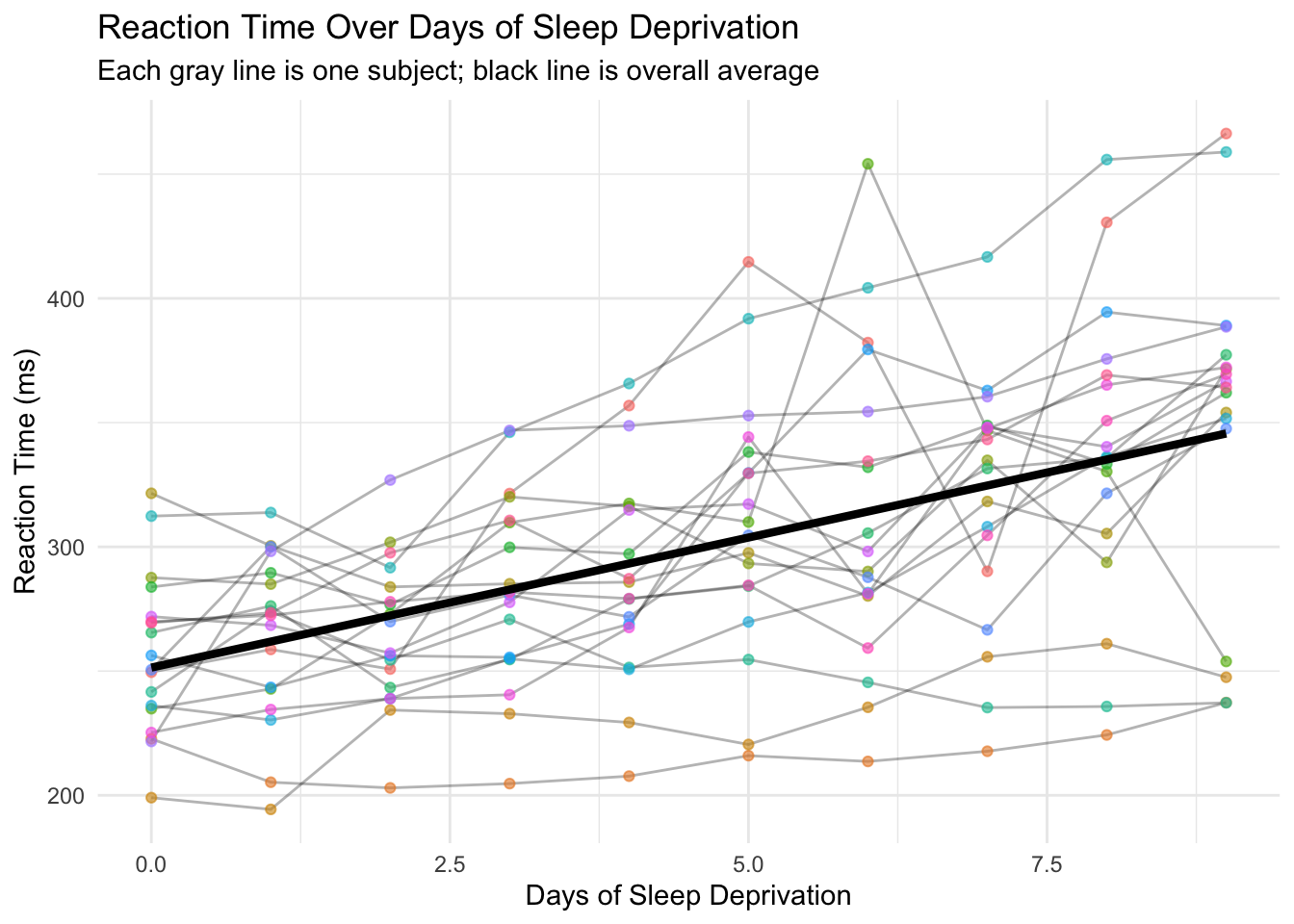
Let's visualize how reaction time changes with sleep deprivation:
```{r}
#| label: fig-individual-trajectories
#| fig-alt: "Scatter plot showing reaction time versus days of sleep deprivation for 18 subjects. Each subject's data points are connected by lines, showing individual trajectories. A black regression line shows the overall trend. Individual patterns vary widely - some subjects show steep increases in reaction time while others remain relatively flat."
# Plot individual trajectories
ggplot(sleepstudy, aes(x = Days, y = Reaction)) +
  geom_line(aes(group = Subject), alpha = 0.3) +
  geom_point(aes(color = Subject), alpha = 0.6) +
  geom_smooth(method = "lm", color = "black", linewidth = 1.5, se = FALSE) +
  labs(
    title = "Reaction Time Over Days of Sleep Deprivation",
    subtitle = "Each gray line is one subject; black line is overall average",
    x = "Days of Sleep Deprivation",
    y = "Reaction Time (ms)"
  ) +
  theme_minimal() +
  theme(legend.position = "none")
```
This plot reveals two important things:
1. **Overall trend**: Reaction times increase with more sleep deprivation (people get slower)
2. **Individual differences**: People start at different baselines AND deteriorate at different rates
Some subjects start slow and get much worse. Others start fast and barely change. A single regression line misses all this individual variation.
### Regular Regression: The Wrong Approach
```{r}
# Fit regular linear regression (WRONG for repeated measures)
model_wrong <- lm(Reaction ~ Days, data = sleepstudy)
summary(model_wrong)
```
This model treats all 180 observations as independent. But they're not - they come from only 18 people! The standard errors are wrong because we're pretending we have 180 independent data points when we really have 18 subjects measured 10 times each.
::: {.callout-warning}
## Don't Do This!
Using `lm()` on repeated measures data inflates your sample size artificially, leading to p-values that are too small and confidence intervals that are too narrow. Your "significant" findings may be false positives.
:::
## Example 1: Random Intercepts Model
### The Idea
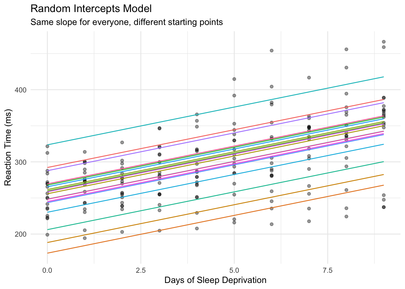
A **random intercepts** model allows each subject to have their own baseline reaction time, while estimating a common slope for how everyone deteriorates with sleep deprivation.
Think of it as: "Everyone slows down by the same amount per day, but some people start faster than others."
::: {.callout-tip}
## Start Simple
Always begin with random intercepts only. Add random slopes later if needed. This approach is more likely to converge and easier to interpret.
:::
### Fitting the Model
```{r}
# Fit mixed effects model with random intercept per subject
model_intercepts <- lmer(Reaction ~ Days + (1 | Subject), data = sleepstudy)
summary(model_intercepts)
```
Breaking down the formula `Reaction ~ Days + (1 | Subject)`:
- `Reaction ~ Days`: Fixed effect - days of sleep deprivation predicts reaction time
- `(1 | Subject)`: Random effect - allow the intercept to vary by subject
### Understanding the Output
**Fixed Effects:**
```{r}
fixef(model_intercepts)
```
- **Intercept (251.4)**: Average reaction time at Day 0 across all subjects
- **Days (10.5)**: For each additional day, reaction time increases by ~10.5 ms on average
**Random Effects:**
```{r}
# See each subject's deviation from the average intercept
ranef(model_intercepts)$Subject |> head()
```
Positive values = subject starts slower than average. Negative values = subject starts faster than average.
### Visualizing Random Intercepts
```{r}
#| label: fig-random-intercepts
#| fig-alt: "Plot showing random intercepts model predictions. Multiple parallel lines with the same slope but different y-intercepts represent each subject. All lines increase at the same rate, but start at different baseline reaction times."
# Get predictions
sleepstudy_pred <- sleepstudy |>
  mutate(
    pred_wrong = predict(model_wrong),
    pred_intercepts = predict(model_intercepts)
  )

# Plot random intercepts model
ggplot(sleepstudy_pred, aes(x = Days, y = Reaction)) +
  geom_point(alpha = 0.4) +
  geom_line(aes(y = pred_intercepts, group = Subject, color = Subject)) +
  labs(
    title = "Random Intercepts Model",
    subtitle = "Same slope for everyone, different starting points",
    x = "Days of Sleep Deprivation",
    y = "Reaction Time (ms)"
  ) +
  theme_minimal() +
  theme(legend.position = "none")
```
Each subject gets their own intercept (starting point), but all lines are parallel - they share the same slope.
## Example 2: Random Slopes Model
### The Problem with Random Intercepts Only
Look back at the individual trajectories plot. Some subjects have steep slopes (deteriorate quickly), others have flat slopes (barely affected by sleep deprivation). The random intercepts model forces everyone to have the same slope - that's too restrictive.
### Fitting Random Slopes
```{r}
# Fit model with random intercepts AND random slopes
model_slopes <- lmer(Reaction ~ Days + (1 + Days | Subject), data = sleepstudy)
summary(model_slopes)
```
The formula `(1 + Days | Subject)` means:
- `1`: Allow intercepts to vary by subject
- `Days`: Allow the slope of Days to vary by subject too
### Understanding Random Slopes Output
**Fixed Effects** (the "average" person):
```{r}
fixef(model_slopes)
```
**Random Effects** (individual deviations):
```{r}
# Each subject's intercept AND slope
coef(model_slopes)$Subject |> head()
```
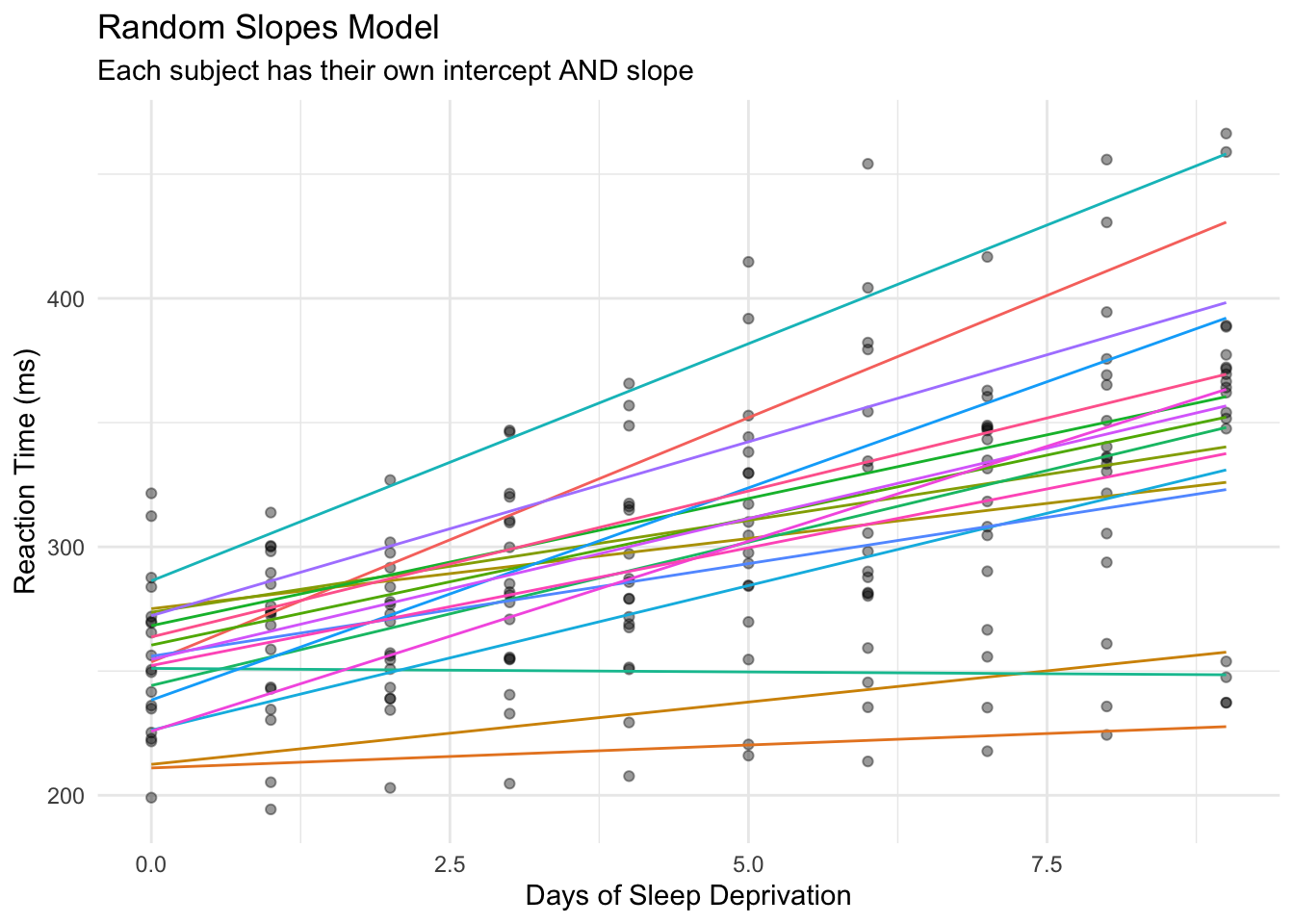
Now each subject has their own intercept AND their own slope. Subject 308 has a slope of ~19.7 (deteriorates quickly), while Subject 309 has a slope of ~1.8 (barely affected).
### Visualizing Random Slopes
```{r}
#| label: fig-random-slopes
#| fig-alt: "Plot showing random slopes model predictions. Multiple lines with different slopes and intercepts represent each subject. Lines are no longer parallel - some subjects show steep increases in reaction time over days while others show minimal change."
# Get predictions from random slopes model
sleepstudy_pred <- sleepstudy_pred |>
  mutate(pred_slopes = predict(model_slopes))

# Plot random slopes model
ggplot(sleepstudy_pred, aes(x = Days, y = Reaction)) +
  geom_point(alpha = 0.4) +
  geom_line(aes(y = pred_slopes, group = Subject, color = Subject)) +
  labs(
    title = "Random Slopes Model",
    subtitle = "Each subject has their own intercept AND slope",
    x = "Days of Sleep Deprivation",
    y = "Reaction Time (ms)"
  ) +
  theme_minimal() +
  theme(legend.position = "none")
```
Now the lines are no longer parallel - each subject has their own trajectory. This better captures the reality of individual differences in sleep deprivation effects.
## Example 3: Model Comparison
We've now fit three different models to the same data:
1. **Regular regression** - ignores that subjects are measured repeatedly
2. **Random intercepts** - allows different starting points, same slope for all
3. **Random slopes** - allows different starting points AND different slopes
But which model should we actually use? This is a critical question because:
- **Too simple** (regular regression): Violates assumptions, gives wrong standard errors
- **Too complex** (random slopes when not needed): Wastes degrees of freedom, may not converge
- **Just right**: Captures the true data structure without over-fitting
We'll use three approaches to decide:
| Method | Question It Answers |
|--------|---------------------|
| **AIC** | Which model balances fit and complexity best? |
| **Likelihood Ratio Test** | Is the more complex model significantly better? |
| **Residual Analysis** | Does the model capture the data structure? |
### Which Model is Best?
Let's compare all three approaches:
```{r}
# Compare models using AIC (lower is better)
AIC(model_wrong, model_intercepts, model_slopes)
```
The random slopes model has the lowest AIC, indicating it's the best fit for this data.
### Likelihood Ratio Test
```{r}
# Formal test: does adding random slopes improve the model?
anova(model_intercepts, model_slopes)
```
The significant p-value confirms that allowing slopes to vary by subject significantly improves the model.
::: {.callout-note}
## Interpreting the Likelihood Ratio Test
The test compares nested models (simpler vs more complex). A significant p-value means the extra complexity is justified - the random slopes capture real variation that random intercepts alone miss.
:::
### Comparing Residuals
```{r}
#| label: fig-residuals-regular
#| fig-alt: "Box plots showing residuals from regular regression grouped by subject. Several subjects show systematic bias - their residuals are consistently above or below zero, indicating the model is missing subject-level patterns."
# Add residuals
sleepstudy_pred <- sleepstudy_pred |>
  mutate(
    resid_wrong = residuals(model_wrong),
    resid_slopes = residuals(model_slopes)
  )

# Plot residuals by subject for wrong model
ggplot(sleepstudy_pred, aes(x = Subject, y = resid_wrong)) +
  geom_boxplot() +
  geom_hline(yintercept = 0, linetype = "dashed", color = "red") +
  labs(
    title = "Regular Regression Residuals by Subject",
    subtitle = "Systematic patterns indicate model is missing subject-level effects",
    y = "Residual"
  ) +
  theme_minimal() +
  theme(axis.text.x = element_text(angle = 45, hjust = 1))
```
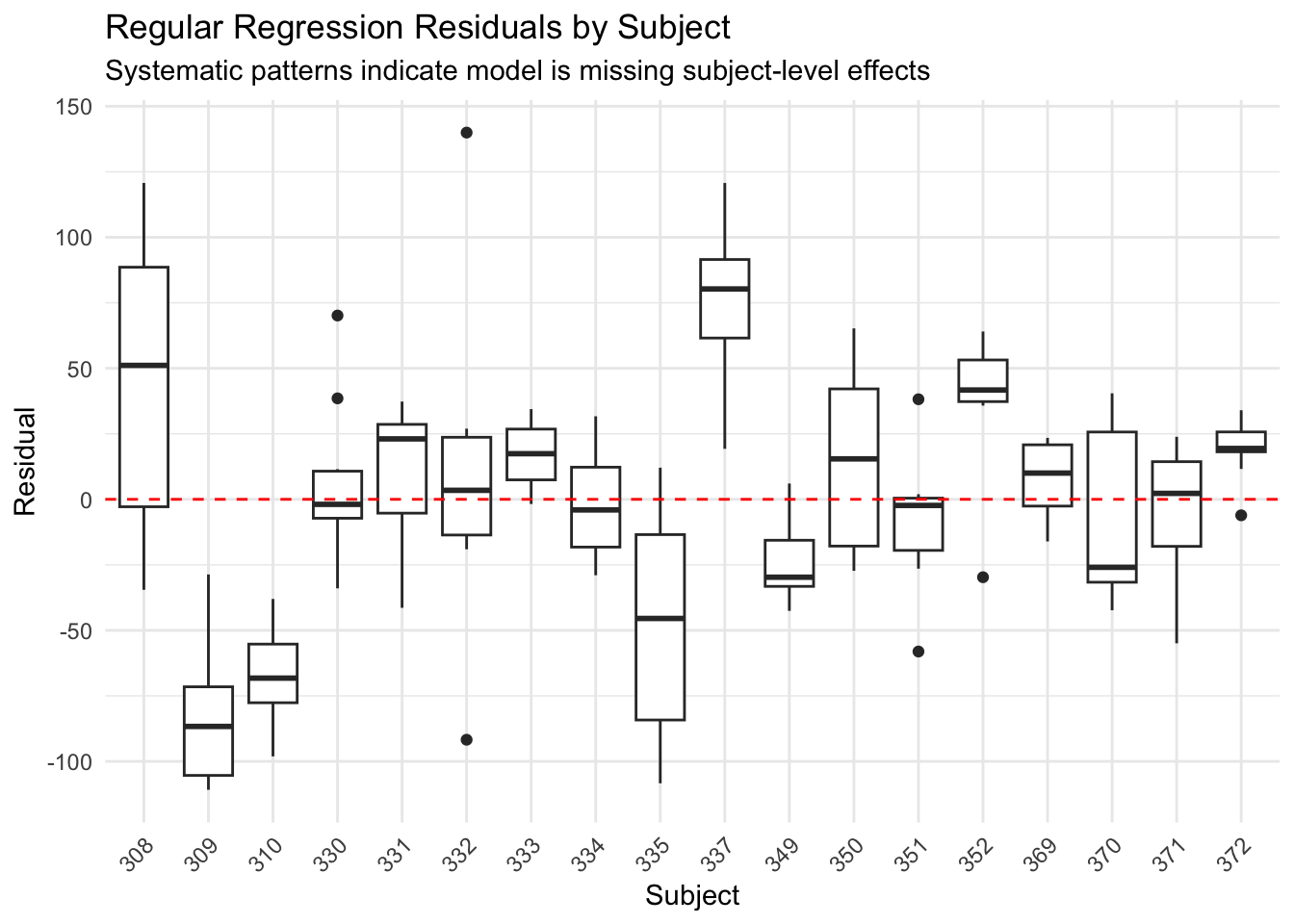
The regular regression shows systematic patterns - some subjects are consistently over or under-predicted. The model is missing the individual differences.
```{r}
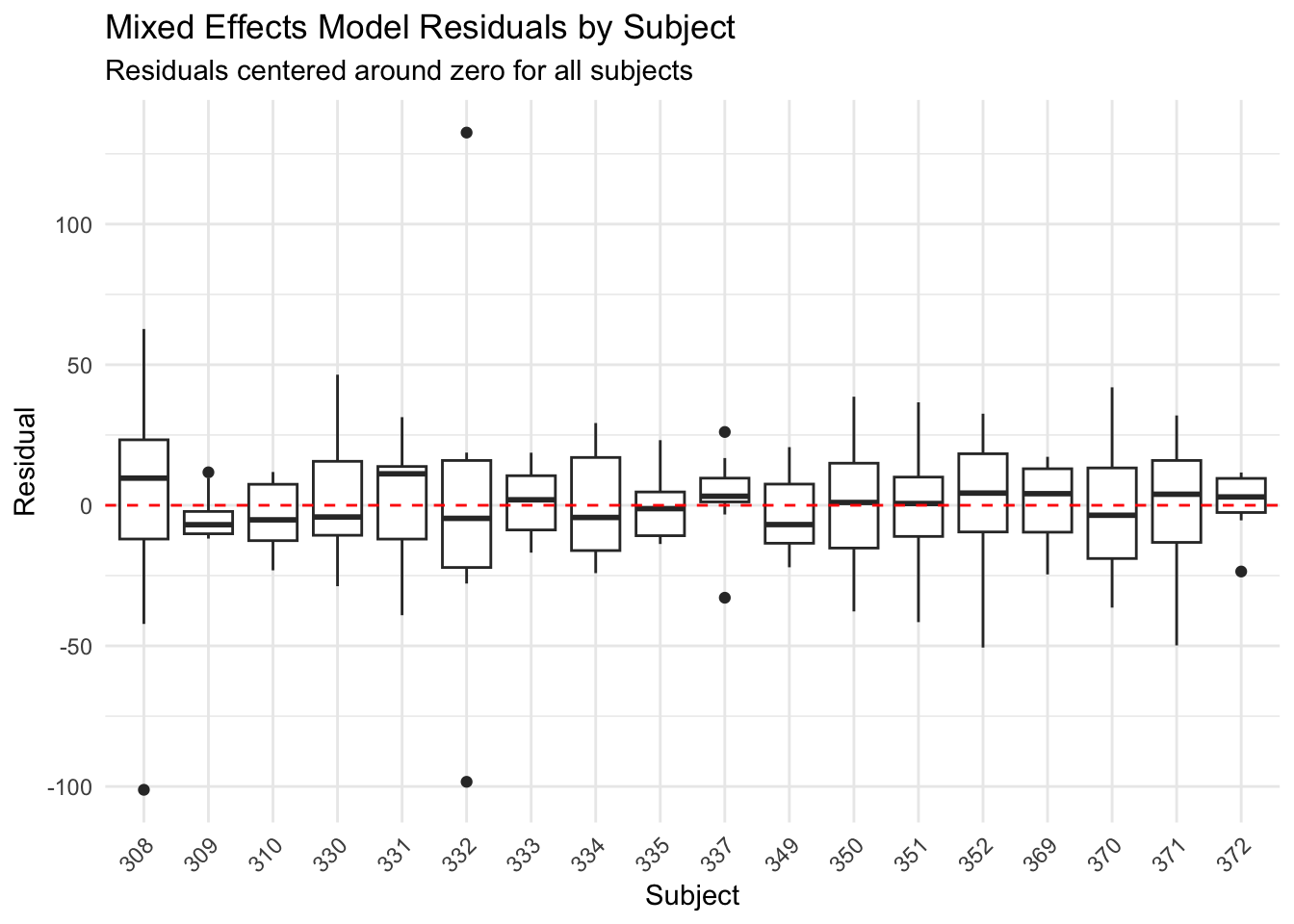
#| label: fig-residuals-mixed
#| fig-alt: "Box plots showing residuals from the mixed effects model grouped by subject. All subjects' residuals are now centered around zero, indicating the model properly accounts for individual differences."
# Plot residuals for mixed model
ggplot(sleepstudy_pred, aes(x = Subject, y = resid_slopes)) +
  geom_boxplot() +
  geom_hline(yintercept = 0, linetype = "dashed", color = "red") +
  labs(
    title = "Mixed Effects Model Residuals by Subject",
    subtitle = "Residuals centered around zero for all subjects",
    y = "Residual"
  ) +
  theme_minimal() +
  theme(axis.text.x = element_text(angle = 45, hjust = 1))
```
The mixed effects model residuals are centered around zero for each subject - we've properly accounted for individual differences.
## Example 4: Making Predictions
### Subject-Specific Predictions
One advantage of mixed models is making predictions for specific subjects:
```{r}
# Predict for a specific subject on a new day
new_data <- data.frame(Days = c(10, 11, 12), Subject = "308")
predict(model_slopes, newdata = new_data)
```
### Population-Level Predictions
For a "typical" new subject, use `re.form = NA` to ignore random effects:
```{r}
# Predict for an average/new subject
new_data_pop <- data.frame(Days = c(10, 11, 12))
predict(model_slopes, newdata = new_data_pop, re.form = NA)
```
## Tidying Results with broom.mixed
The [`broom.mixed`](https://cran.r-project.org/package=broom.mixed) package makes it easy to extract model results in tidy data frames - perfect for reporting or further analysis.
### Tidy Fixed Effects
```{r}
# Get fixed effects as a tidy data frame
tidy(model_slopes, effects = "fixed")
```
This gives you estimates, standard errors, and confidence intervals in a format ready for tables or plotting.
### Tidy Random Effects
```{r}
# Get random effects (subject-level deviations)
tidy(model_slopes, effects = "ran_vals") |> head(10)
```
### Model Summary Statistics
```{r}
# Get model-level statistics (AIC, BIC, etc.)
glance(model_slopes)
```
### Augmented Data with Predictions
```{r}
# Add predictions and residuals to your data
augment(model_slopes) |> head()
```
The `.fitted` column contains predictions, and `.resid` contains residuals - useful for diagnostics or visualization.
::: {.callout-tip}
## Why Use broom.mixed?
Base R's `summary()` prints results to the console. `broom.mixed` returns data frames you can filter, join, or pass to ggplot2. This is especially useful when comparing multiple models or creating publication-ready tables.
:::
## When to Use Mixed Effects Models
| Situation | Example | Random Effect |
|-----------|---------|---------------|
| **Longitudinal data** | Same people measured over time | Subject |
| **[Repeated measures](/statistics/how-to-repeated-measures-anova-in-r.html)** | Multiple trials per person | Subject |
| **Clustered data** | Students within schools | School |
| **Nested designs** | Patients within hospitals within regions | Hospital, Region |
| **Crossed designs** | Subjects rating multiple items | Subject, Item |
## Common Mistakes to Avoid
**1. Treating repeated measures as independent** (see [linear regression basics](/statistics/how-to-linear-regression-basics-in-r.html) for when simple regression IS appropriate)
```r
# WRONG: Ignores that measurements come from the same subjects
lm(Reaction ~ Days, data = sleepstudy)

# RIGHT: Accounts for within-subject correlation
lmer(Reaction ~ Days + (1 | Subject), data = sleepstudy)
```
**2. Starting with too complex a model**
Start with random intercepts only. Add random slopes if:
- Theory suggests the effect varies across subjects
- You have enough data (5+ observations per subject)
- The simpler model shows poor fit
**3. Ignoring convergence warnings**
If you see warnings, simplify your model:
```r
# Too complex - may not converge
lmer(y ~ x1 + x2 + x3 + (1 + x1 + x2 + x3 | Subject), data = df)

# Simpler - more likely to converge
lmer(y ~ x1 + x2 + x3 + (1 + x1 | Subject), data = df)
```
## Quick Reference: Formula Syntax
::: {.callout-note appearance="minimal"}
## lme4 Formula Cheatsheet
| Formula | Meaning | Use When |
|---------|---------|----------|
| `y ~ x + (1 | group)` | Random intercepts only | Groups differ in baseline |
| `y ~ x + (1 + x | group)` | Random intercepts + slopes | Groups differ in baseline AND effect of x |
| `y ~ x + (0 + x | group)` | Random slopes only (no intercept) | Rare; baseline is fixed but slopes vary |
| `y ~ x + (1 | group1) + (1 | group2)` | Crossed random effects | Two grouping factors (e.g., subjects AND items) |
| `y ~ x + (1 | group1/group2)` | Nested random effects | group2 is nested within group1 |
| `y ~ x + (1 | group) + (0 + x | group)` | Uncorrelated random effects | When correlated version won't converge |
**Key functions:**
```r
lmer(formula, data)      # Fit linear mixed model
summary(model)           # View full output
fixef(model)             # Extract fixed effects
ranef(model)             # Extract random effects (deviations)
coef(model)              # Extract coefficients per group
predict(model)           # Get fitted values
AIC(model1, model2)      # Compare model fit
anova(model1, model2)    # Likelihood ratio test
```
:::
## Summary
- **Regular regression** treats all observations as independent - wrong for repeated measures
- **Mixed effects models** account for the correlation within subjects
- **Random intercepts** `(1 | Subject)`: Subjects differ in their baseline
- **Random slopes** `(1 + x | Subject)`: Subjects differ in how they respond to x
- The `sleepstudy` data shows both: people start at different baselines AND deteriorate at different rates
- Use `lmer()` from `lme4` for continuous outcomes
- Compare models with `AIC()` and `anova()`
- Always visualize individual trajectories to understand your data
---
## Frequently Asked Questions
**Q: What's the difference between mixed effects models and repeated measures ANOVA?**
Both handle repeated measurements, but mixed effects models are more flexible. They handle unbalanced designs (missing data), continuous predictors, and can model how the effect itself varies across subjects. [Repeated measures ANOVA](/statistics/how-to-repeated-measures-anova-in-r.html) is a special case of mixed models.
**Q: How many subjects do I need for a mixed effects model?**
A common rule of thumb is at least 5-10 groups (subjects) for random intercepts, and more for random slopes. With too few groups, random effects estimates become unstable. If you have only 3-4 subjects, consider treating subject as a fixed effect instead.
**Q: How many measurements per subject do I need?**
For random intercepts only, even 2-3 measurements per subject can work. For random slopes, you need enough observations per subject to estimate individual slopes - typically 4-5+ time points. In the sleepstudy data, 10 measurements per subject allows reliable estimation of both intercepts and slopes. More observations per subject = better individual-level estimates; more subjects = better population-level estimates.
**Q: My model won't converge. What should I do?**
Convergence issues usually mean your model is too complex for your data. Try:
1. Remove random slopes and keep only random intercepts
2. Remove correlation between random effects: `(1 | Subject) + (0 + Days | Subject)`
3. Scale your predictors using `scale()`
4. Check for outliers or data entry errors
**Q: Should I use `lme4` or `nlme` for mixed models?**
[`lme4`](https://cran.r-project.org/package=lme4) is generally preferred for modern analyses. It's faster, handles crossed random effects better, and integrates well with the tidyverse. Use [`nlme`](https://cran.r-project.org/package=nlme) if you need specific correlation structures or heterogeneous variances.
**Q: How do I get p-values for fixed effects?**
`lme4` deliberately doesn't provide p-values because calculating degrees of freedom for mixed models is complex. Options include:
- Use the [`lmerTest`](https://cran.r-project.org/package=lmerTest) package which adds p-values via Satterthwaite approximation
- Use likelihood ratio tests with `anova()`
- Use confidence intervals: if 95% CI doesn't include zero, effect is "significant"
**Q: Can I use mixed models for binary outcomes?**
Yes! Use `glmer()` instead of `lmer()` with `family = binomial`. For example: `glmer(success ~ treatment + (1 | subject), family = binomial, data = df)`. See our [logistic regression guide](/statistics/how-to-logistic-regression-in-r.html) for background on binary outcomes.
---
## Further Reading
- [lme4 package documentation](https://cran.r-project.org/package=lme4) - The standard R package for mixed effects models
- [lme4 vignette: Fitting Linear Mixed-Effects Models](https://cran.r-project.org/web/packages/lme4/vignettes/lmer.pdf) - Official guide by the package authors
- [broom.mixed package](https://cran.r-project.org/package=broom.mixed) - Tidy output from mixed models
- [GLMM FAQ](https://bbolker.github.io/mixedmodels-misc/glmmFAQ.html) - Comprehensive FAQ by Ben Bolker (lme4 co-author)
## Related Posts
- [How to linear regression basics in R](/statistics/how-to-linear-regression-basics-in-r.html)
- [How to ANOVA one-way in R](/statistics/how-to-anova-one-way-in-r.html)
- [How to ANOVA two-way in R](/statistics/how-to-anova-two-way-in-r.html)
- [How to multiple linear regression in R](/statistics/how-to-multiple-linear-regression-in-r.html)
- [How to repeated measures ANOVA in R](/statistics/how-to-repeated-measures-anova-in-r.html)